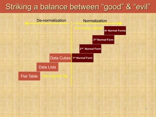
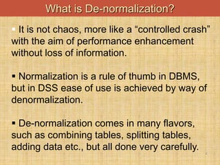
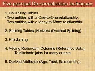
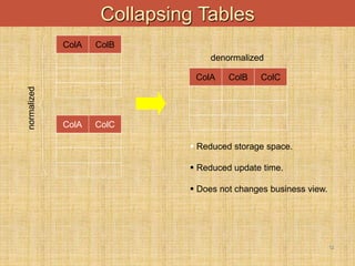
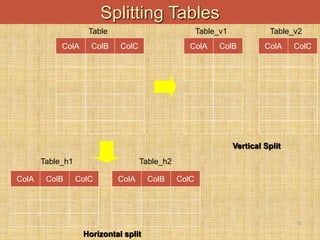
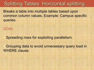
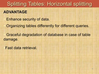
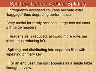
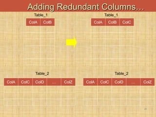
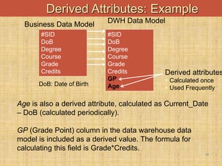
Data Warehousing
De-normalization
1
Ch Anwar ul Hassan (Lecturer)
Department of Computer Science and Software
Engineering
Capital University of Sciences & Technology, Islamabad
Pakistan
anwarchaudary@gmail.com
2
Striking a balance between “good” & “evil”
Flat Table
Data Lists
Data Cubes 1st Normal Form
2nd Normal Form
3rd Normal Form
4+ Normal Forms
NormalizationDe-normalization
One big flat file
Too many tables
3
What is De-normalization?
 It is not chaos, more like a “controlled crash”
with the aim of performance enhancement
without loss of information.
 Normalization is a rule of thumb in DBMS,
but in DSS ease of use is achieved by way of
denormalization.
 De-normalization comes in many flavors,
such as combining tables, splitting tables,
adding data etc., but all done very carefully.
4
Why De-normalization In DSS?
 Bringing “close” dispersed but related data
items.
 Query performance in DSS significantly
dependent on physical data model.
 Very early studies showed performance
difference in orders of magnitude for different
number de-normalized tables and rows per table.
 The level of de-normalization should be
carefully considered.
5
How De-normalization improves performance?
De-normalization specifically improves
performance by either:
 Reducing the number of tables and hence the
reliance on joins, which consequently speeds up
performance.
 Reducing the number of joins required during
query execution
 Reducing the number of rows to be retrieved from
the Primary Data Table.
6
4 Guidelines for De-normalization
1. Carefully do a cost-benefit analysis
(frequency of use, additional storage,
join time).
2. Do a data requirement and storage
analysis.
3. Weigh against the maintenance issue
of the redundant data (triggers used).
4. When in doubt, don’t denormalize.
7
Areas for Applying De-Normalization Techniques
 Dealing with the abundance of star schemas.
 Fast access of time series data for analysis.
 Fast aggregate (sum, average etc.) results and
complicated calculations.
 Multidimensional analysis (e.g. geography) in a complex
hierarchy.
 Dealing with few updates but many join queries.
De-normalization will ultimately affect the database size and
query performance.
 Star Schema, the center of the star can have one fact table and a
number of associated dimension tables. It is known as star schema
as its structure resembles a star. The star schema is the simplest
type of Data Warehouse schema. It is also known as Star Join
Schema and is optimized for querying large data sets.
8
Star Schema
 Snowflake Schema is an extension of a Star Schema,
and it adds additional dimensions. It is called snowflake
because its diagram resembles a Snowflake.
9
Star Schema
10
Five principal De-normalization techniques
1. Collapsing Tables.
- Two entities with a One-to-One relationship.
- Two entities with a Many-to-Many relationship.
2. Splitting Tables (Horizontal/Vertical Splitting).
3. Pre-Joining.
4. Adding Redundant Columns (Reference Data).
To eliminate joins for many queries
5. Derived Attributes (Age, Total, Balance etc).
11
De-normalization Techniques
12
Collapsing Tables
ColA ColB
ColA ColC
normalized
ColA ColB ColC
denormalized
 Reduced storage space.
 Reduced update time.
 Does not changes business view.
13
Splitting Tables
ColA ColB ColC
Table
Vertical Split
ColA ColB ColA ColC
Table_v1 Table_v2
ColA ColB ColC
Horizontal split
ColA ColB ColC
Table_h1 Table_h2
14
Splitting Tables: Horizontal splitting…
Breaks a table into multiple tables based upon
common column values. Example: Campus specific
queries.
GOAL
 Spreading rows for exploiting parallelism.
 Grouping data to avoid unnecessary query load in
WHERE clause.
15
Splitting Tables: Horizontal splitting
ADVANTAGE
 Enhance security of data.
 Organizing tables differently for different queries.
 Graceful degradation of database in case of table
damage.
Fast data retrieval.
16
Splitting Tables: Vertical Splitting
 Infrequently accessed columns become extra
“baggage” thus degrading performance.
Very useful for rarely accessed large text columns
with large headers.
 Header size is reduced, allowing more rows per
block, thus reducing I/O.
Splitting and distributing into separate files with
repeating primary key.
 For an end user, the split appears as a single table
through a view.
17
Pre-joining …
 Identify frequent joins and append the tables
together in the physical data model.
 Generally used for 1:M such as master-
detail.
 Additional space is required as the master
information is repeated in the new header
table.
18
Pre-Joining…
normalized
Tx_ID Sale_ID Item_ID Item_Qty Sale_Rs
Tx_ID Sale_ID Item_ID Item_Qty Sale_RsSale_dateSale_person
denormalized
Sale_IDSale_dateSale_person
Master
Detail
1 M
19
Pre-Joining: Typical Scenario
 Typical of Market basket query
 Join ALWAYS required
 Tables could be millions of rows
 Squeeze Master into Detail
 Repetition of facts. How much?
 Detail 3-4 times of master
20
Adding Redundant Columns…
ColA ColB
Table_1
ColA ColC ColD … ColZ
Table_2
ColA ColB
Table_1’
ColA ColC ColD … ColZ
Table_2
ColC
21
Adding Redundant Columns…
Columns can also be moved, instead of making them
redundant. Very similar to pre-joining as discussed
earlier.
EXAMPLE
Frequent referencing of code in one table and
corresponding description in another table.
 A join is required.

22
Derived Attributes: Example
Age is also a derived attribute, calculated as Current_Date
– DoB (calculated periodically).
GP (Grade Point) column in the data warehouse data
model is included as a derived value. The formula for
calculating this field is Grade*Credits.
#SID
DoB
Degree
Course
Grade
Credits
Business Data Model
#SID
DoB
Degree
Course
Grade
Credits
GP
Age
DWH Data Model
Derived attributes
 Calculated once
 Used Frequently
DoB: Date of Birth

Intro to Data warehousing Lecture 04

  • 1.
    Data Warehousing De-normalization 1 Ch Anwarul Hassan (Lecturer) Department of Computer Science and Software Engineering Capital University of Sciences & Technology, Islamabad Pakistan anwarchaudary@gmail.com
  • 2.
    2 Striking a balancebetween “good” & “evil” Flat Table Data Lists Data Cubes 1st Normal Form 2nd Normal Form 3rd Normal Form 4+ Normal Forms NormalizationDe-normalization One big flat file Too many tables
  • 3.
    3 What is De-normalization? It is not chaos, more like a “controlled crash” with the aim of performance enhancement without loss of information.  Normalization is a rule of thumb in DBMS, but in DSS ease of use is achieved by way of denormalization.  De-normalization comes in many flavors, such as combining tables, splitting tables, adding data etc., but all done very carefully.
  • 4.
    4 Why De-normalization InDSS?  Bringing “close” dispersed but related data items.  Query performance in DSS significantly dependent on physical data model.  Very early studies showed performance difference in orders of magnitude for different number de-normalized tables and rows per table.  The level of de-normalization should be carefully considered.
  • 5.
    5 How De-normalization improvesperformance? De-normalization specifically improves performance by either:  Reducing the number of tables and hence the reliance on joins, which consequently speeds up performance.  Reducing the number of joins required during query execution  Reducing the number of rows to be retrieved from the Primary Data Table.
  • 6.
    6 4 Guidelines forDe-normalization 1. Carefully do a cost-benefit analysis (frequency of use, additional storage, join time). 2. Do a data requirement and storage analysis. 3. Weigh against the maintenance issue of the redundant data (triggers used). 4. When in doubt, don’t denormalize.
  • 7.
    7 Areas for ApplyingDe-Normalization Techniques  Dealing with the abundance of star schemas.  Fast access of time series data for analysis.  Fast aggregate (sum, average etc.) results and complicated calculations.  Multidimensional analysis (e.g. geography) in a complex hierarchy.  Dealing with few updates but many join queries. De-normalization will ultimately affect the database size and query performance.
  • 8.
     Star Schema,the center of the star can have one fact table and a number of associated dimension tables. It is known as star schema as its structure resembles a star. The star schema is the simplest type of Data Warehouse schema. It is also known as Star Join Schema and is optimized for querying large data sets. 8 Star Schema
  • 9.
     Snowflake Schemais an extension of a Star Schema, and it adds additional dimensions. It is called snowflake because its diagram resembles a Snowflake. 9 Star Schema
  • 10.
    10 Five principal De-normalizationtechniques 1. Collapsing Tables. - Two entities with a One-to-One relationship. - Two entities with a Many-to-Many relationship. 2. Splitting Tables (Horizontal/Vertical Splitting). 3. Pre-Joining. 4. Adding Redundant Columns (Reference Data). To eliminate joins for many queries 5. Derived Attributes (Age, Total, Balance etc).
  • 11.
  • 12.
    12 Collapsing Tables ColA ColB ColAColC normalized ColA ColB ColC denormalized  Reduced storage space.  Reduced update time.  Does not changes business view.
  • 13.
    13 Splitting Tables ColA ColBColC Table Vertical Split ColA ColB ColA ColC Table_v1 Table_v2 ColA ColB ColC Horizontal split ColA ColB ColC Table_h1 Table_h2
  • 14.
    14 Splitting Tables: Horizontalsplitting… Breaks a table into multiple tables based upon common column values. Example: Campus specific queries. GOAL  Spreading rows for exploiting parallelism.  Grouping data to avoid unnecessary query load in WHERE clause.
  • 15.
    15 Splitting Tables: Horizontalsplitting ADVANTAGE  Enhance security of data.  Organizing tables differently for different queries.  Graceful degradation of database in case of table damage. Fast data retrieval.
  • 16.
    16 Splitting Tables: VerticalSplitting  Infrequently accessed columns become extra “baggage” thus degrading performance. Very useful for rarely accessed large text columns with large headers.  Header size is reduced, allowing more rows per block, thus reducing I/O. Splitting and distributing into separate files with repeating primary key.  For an end user, the split appears as a single table through a view.
  • 17.
    17 Pre-joining …  Identifyfrequent joins and append the tables together in the physical data model.  Generally used for 1:M such as master- detail.  Additional space is required as the master information is repeated in the new header table.
  • 18.
    18 Pre-Joining… normalized Tx_ID Sale_ID Item_IDItem_Qty Sale_Rs Tx_ID Sale_ID Item_ID Item_Qty Sale_RsSale_dateSale_person denormalized Sale_IDSale_dateSale_person Master Detail 1 M
  • 19.
    19 Pre-Joining: Typical Scenario Typical of Market basket query  Join ALWAYS required  Tables could be millions of rows  Squeeze Master into Detail  Repetition of facts. How much?  Detail 3-4 times of master
  • 20.
    20 Adding Redundant Columns… ColAColB Table_1 ColA ColC ColD … ColZ Table_2 ColA ColB Table_1’ ColA ColC ColD … ColZ Table_2 ColC
  • 21.
    21 Adding Redundant Columns… Columnscan also be moved, instead of making them redundant. Very similar to pre-joining as discussed earlier. EXAMPLE Frequent referencing of code in one table and corresponding description in another table.  A join is required. 
  • 22.
    22 Derived Attributes: Example Ageis also a derived attribute, calculated as Current_Date – DoB (calculated periodically). GP (Grade Point) column in the data warehouse data model is included as a derived value. The formula for calculating this field is Grade*Credits. #SID DoB Degree Course Grade Credits Business Data Model #SID DoB Degree Course Grade Credits GP Age DWH Data Model Derived attributes  Calculated once  Used Frequently DoB: Date of Birth