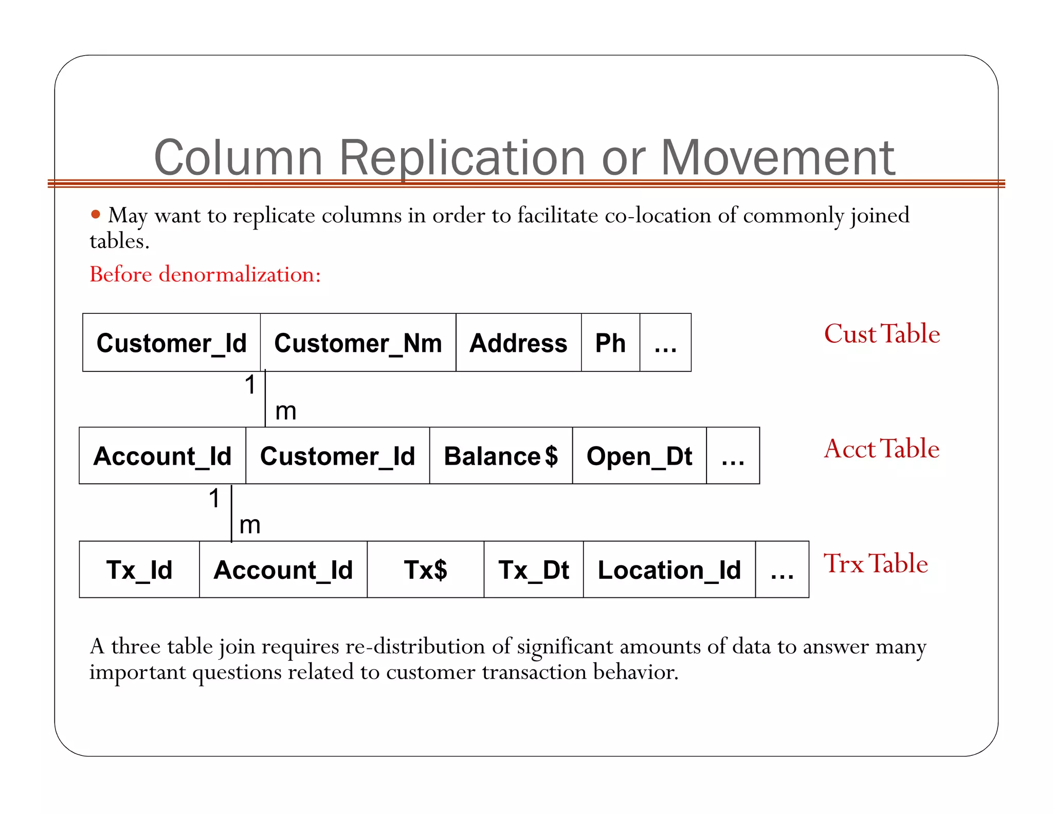
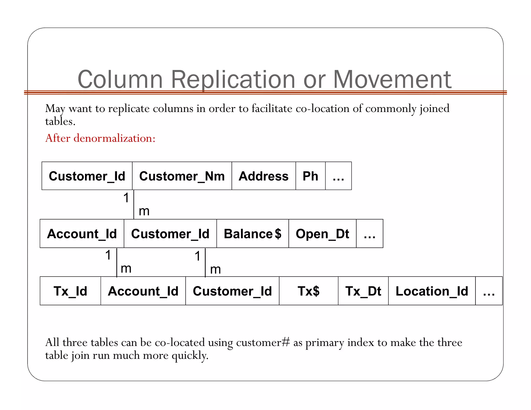
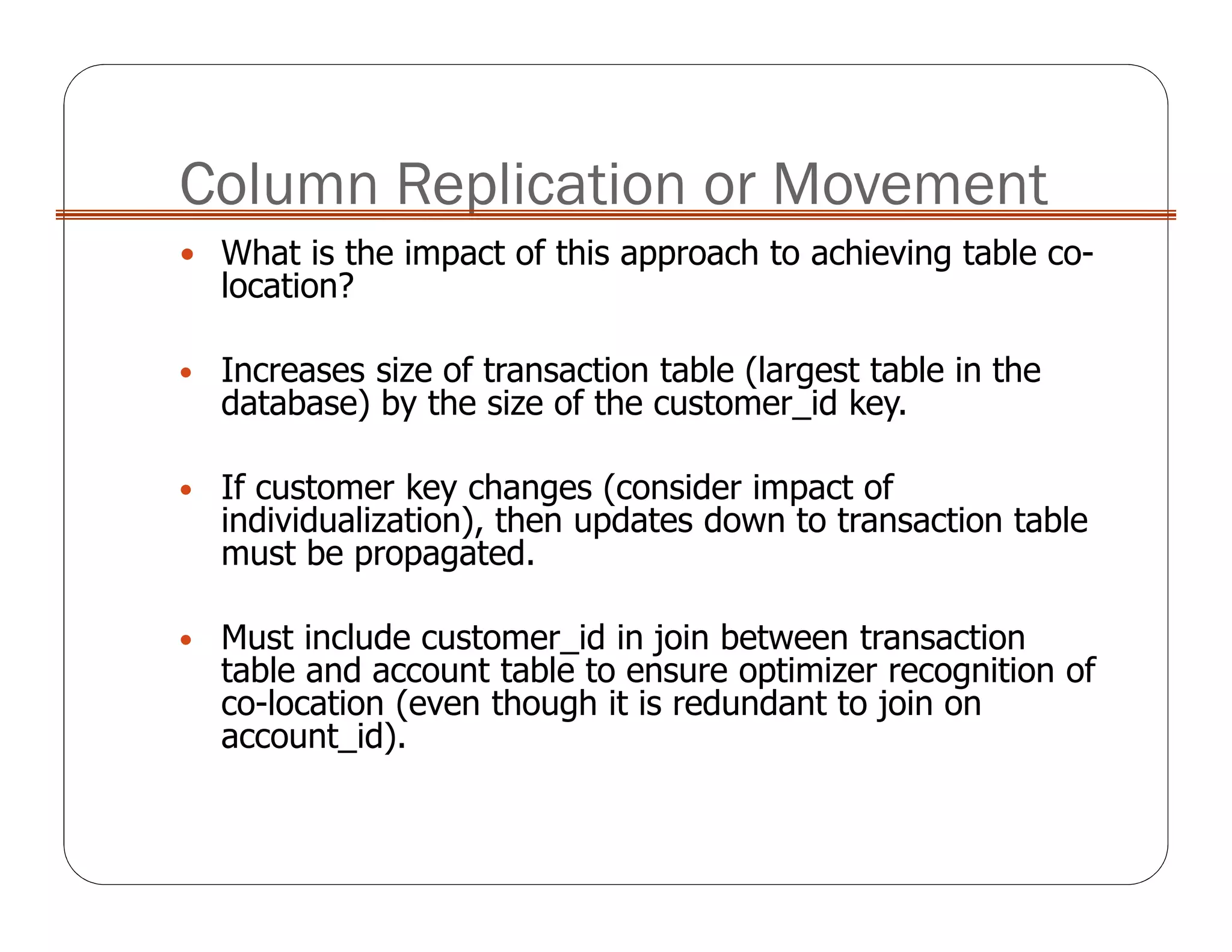
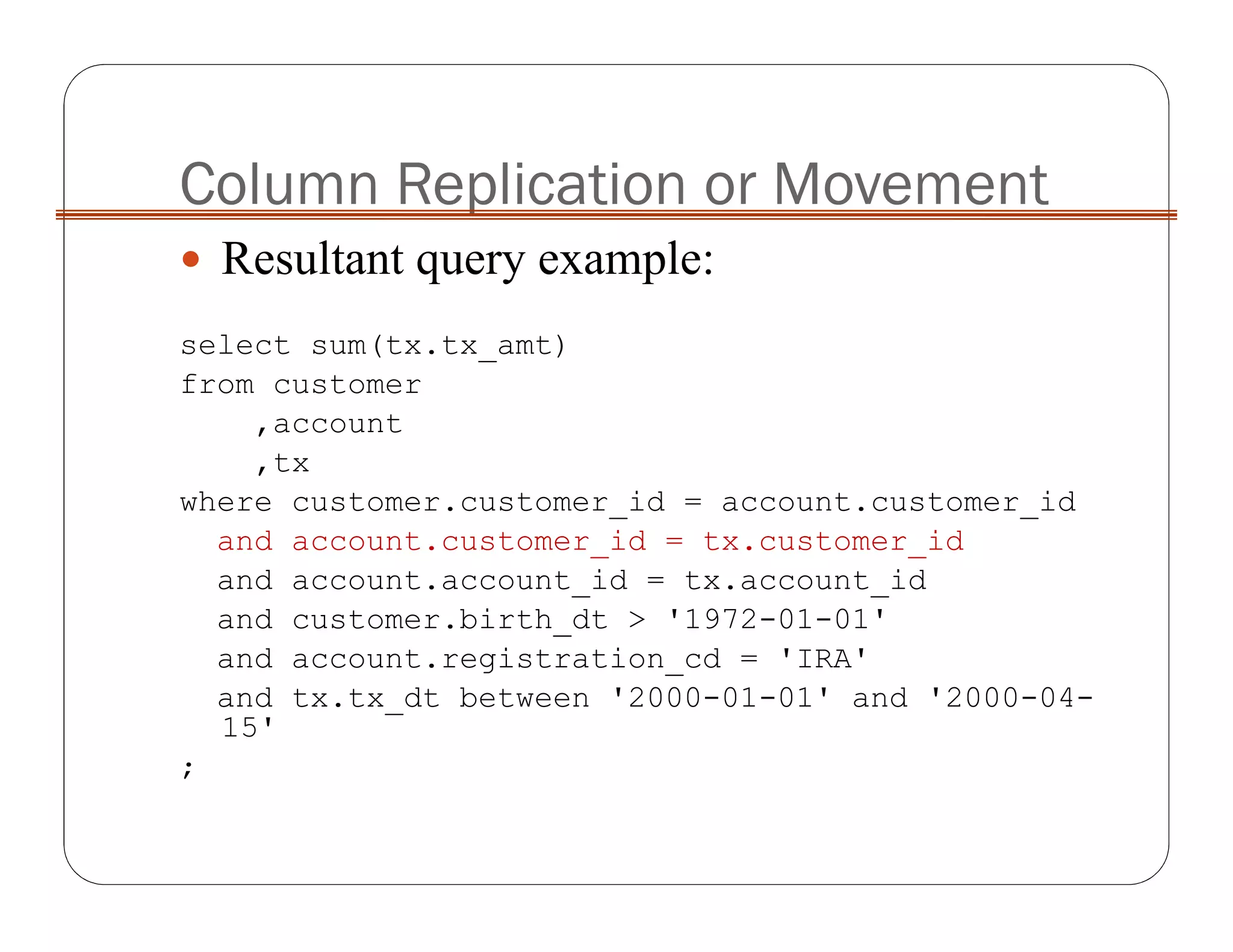
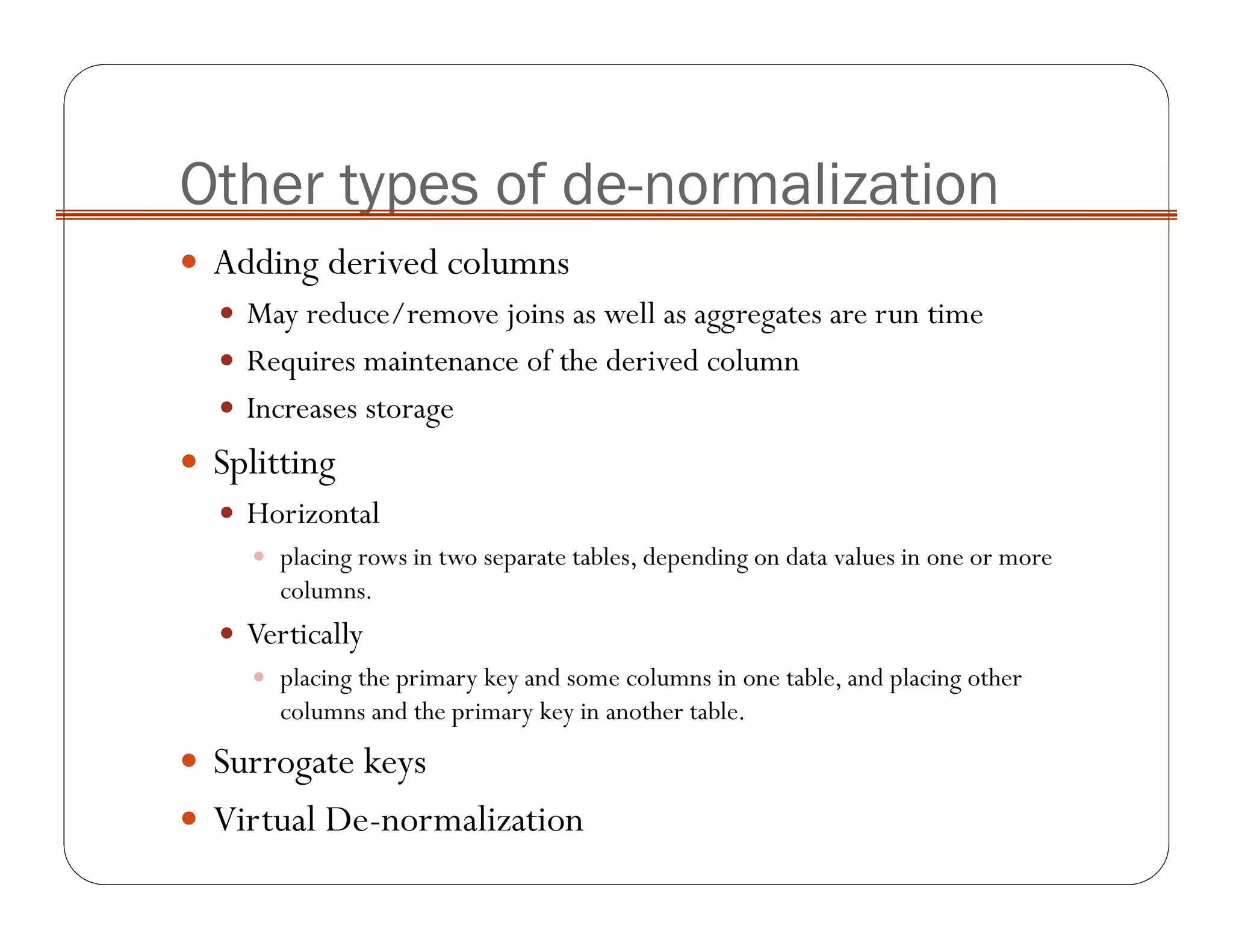
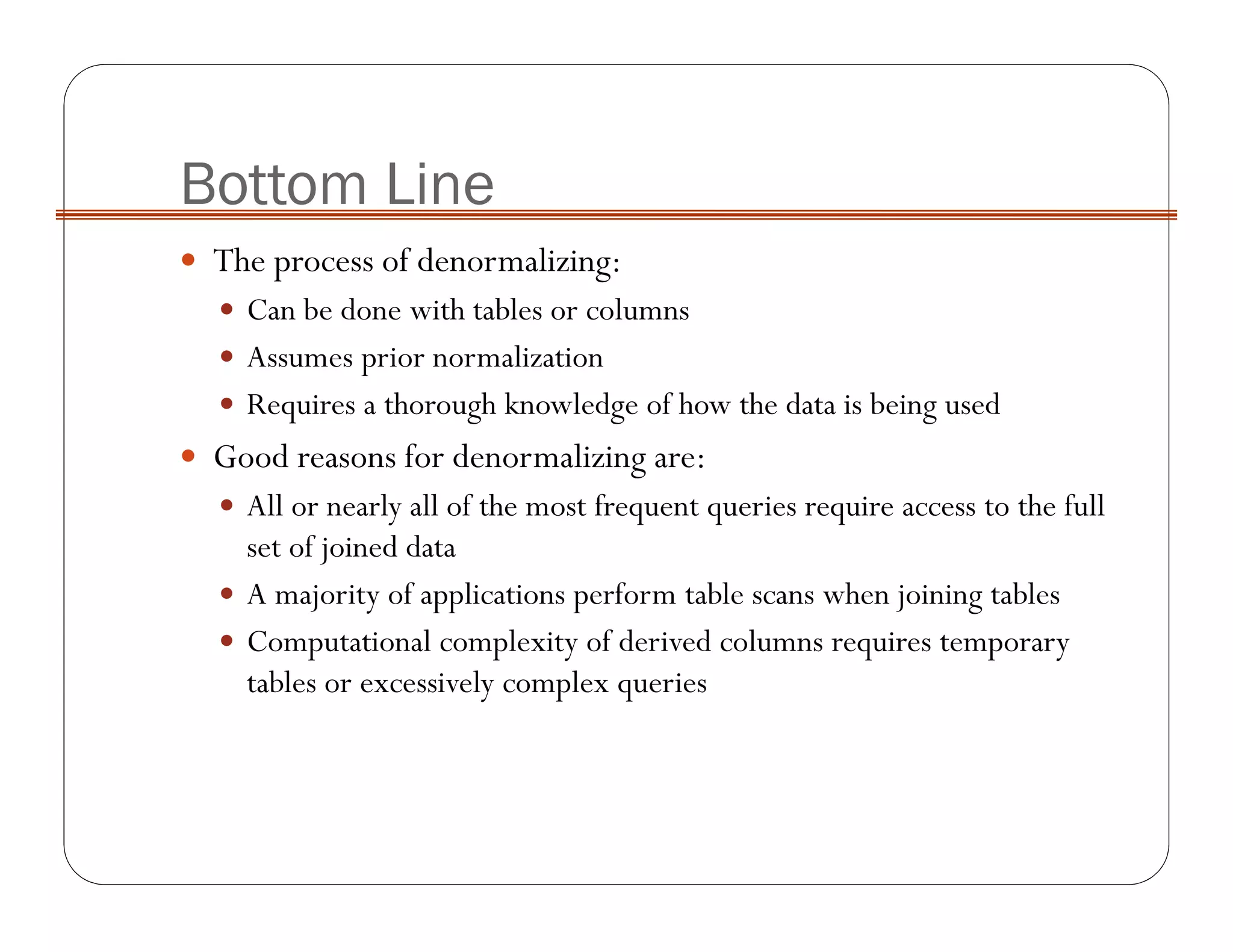
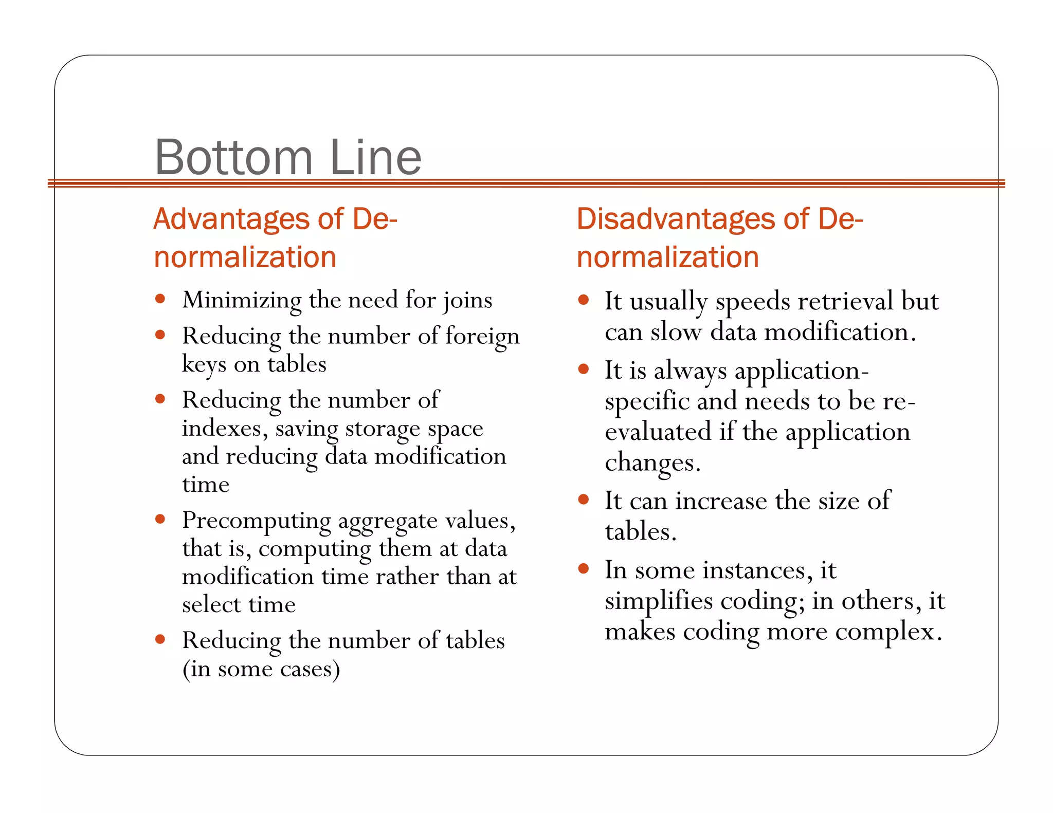
Column Replication or Movement
May want to replicate columns in order to facilitate co-location of commonly joined
tables.
Before denormalization:
A three table join requires re-distribution of significant amounts of data to answer many
important questions related to customer transaction behavior.
Customer_Id Customer_Nm Address Ph …
Account_Id Customer_Id Balance$ Open_Dt …
Tx_Id Account_Id Tx$ Tx_Dt Location_Id …
1
m
1
m
CustTable
AcctTable
TrxTable
Column Replication or Movement
May want to replicate columns in order to facilitate co-location of commonly joined
tables.
After denormalization:
All three tables can be co-located using customer# as primary index to make the three
table join run much more quickly.
Customer_Id Customer_Nm Address Ph …
Account_Id Customer_Id Balance$ Open_Dt …
Tx_Id Account_Id Customer_Id Tx$ Tx_Dt Location_Id …
1
m
1
m
1
m
Column Replication or Movement
What is the impact of this approach to achieving table co-
location?
• Increases size of transaction table (largest table in the
database) by the size of the customer_id key.
• If customer key changes (consider impact of
individualization), then updates down to transaction table
must be propagated.
• Must include customer_id in join between transaction
table and account table to ensure optimizer recognition of
co-location (even though it is redundant to join on
account_id).
Column Replication or Movement
Resultant query example:
select sum(tx.tx_amt)
from customer
,account
,tx
where customer.customer_id = account.customer_id
and account.customer_id = tx.customer_id
and account.account_id = tx.account_id
and customer.birth_dt > '1972-01-01'
and account.registration_cd = 'IRA'
and tx.tx_dt between '2000-01-01' and '2000-04-
15'
;
Pre-aggregation
Take aggregate values that are frequently used in decision-making
and pre-compute them into physical tables in the database.
Can provide huge performance advantage in avoiding frequent
aggregation of detailed data.
Storage implications are usually small compared to size of detailed
data - but can be very large if many multi-dimensional summaries
are constructed.
Pre-aggregation
Ease-of-use for data warehouse can be significantly increased with
selective pre-aggregation.
Pre-aggregation adds significant burden to maintenance for DW.
Pre-aggregation
Typical pre-aggregate summary tables:
Retail: Inventory on hand, sales revenue, cost of goods sold, quantity of good sold,
etc. by store, item, and week.
Healthcare: Effective membership by member age and gender, product, network,
and month.
Telecommunications: Toll call activity in time slot and destination region buckets by
customer and month.
Financial Services: First DOE, last DOE, first DOI, last DOI, rolling $ and
transaction volume in account type buckets, etc. by household.
Transportation: Transaction quantity and $ by customer, source, destination, class of
service, and month.
Pre-aggregation
Standardized definitions for aggregates are critical...
Need business agreement on aggregate definitions.
e.g., accounting period vs. calendar month vs. billing cycle
Must ensure stability in aggregate definitions to provide value in
historical analysis.
Pre-aggregation
Overhead for maintaining aggregates should not be under estimated.
Can choose transactional update strategy or re-build strategy for
maintaining aggregates.
Choice depends on volatility of aggregates and ability to segregate
aggregate records that need to be refreshed based on incoming
data.
e.g., customer aggregates vs. weekly POS activity aggregates.
Cost of updating an aggregate record is typically ten times higher
than the cost of inserting a new record in a detail table
(transactional update cost versus bulk loading cost).
Pre-aggregation
An aggregate table must be used many, many times per day to
justify its existence in terms of maintenance overhead in most
environments.
Consider views if primary motivation is ease-of-use as opposed to
a need for performance enhancement.
Pre-aggregation
Aggregates should NOT replace detailed data.
Aggregates enhance performance and usability for accessing pre-
defined views of the data.
Detailed data will still be required for ad hoc and more
sophisticated analyses.
Other types of de-normalization
Adding derived columns
May reduce/remove joins as well as aggregates are run time
Requires maintenance of the derived column
Increases storage
Splitting
Horizontal
placing rows in two separate tables, depending on data values in one or more
columns.
Vertically
placing the primary key and some columns in one table, and placing other
columns and the primary key in another table.
Surrogate keys
Virtual De-normalization
Derived Attributes
Age is also a derived attribute, calculated as Current_Date – DoB
(calculated periodically).
GP (Grade Point) column in the data warehouse data model is included as
a derived value.The formula for calculating this field is Grade*Credits.
#SID
DoB
Degree
Course
Grade
Credits
Business Data
Model
#SID
DoB
Degree
Course
Grade
Credits
GP
Age
DWH Data Model
DoB: Date of Birth
ColA ColB ColC
Table
Vertical Split
ColA ColB ColA ColC
Table_v1 Table_v2
ColA ColB ColC
Horizontal split
ColA ColB ColC
Table_h1 Table_h2
Splitting
Bottom Line
In a perfect world of infinitely fast machines and well-designed end
user access tools, de-normalization would never be discussed.
In the reality in which we design very large databases, selective
denormalization is usually required - but it is important to initiate the
design from a clean (normalized) starting point.
A good approach is to normalize your data (to 3NF) and then perform
selective denormalization if and when required by performance issues.
Denormalization is NOT “total chaos” but more like a controlled crash.
Bottom Line
When a table is normalized, the non-key columns depend on the
key, the whole key, and nothing but the key.
In order to denormalize, you should have very good knowledge of
the underlying database schema.
Need to be acutely aware of storage and maintenance costs
associated with de-normalization techniques.
Bottom Line
The process of denormalizing:
Can be done with tables or columns
Assumes prior normalization
Requires a thorough knowledge of how the data is being used
Good reasons for denormalizing are:
All or nearly all of the most frequent queries require access to the full
set of joined data
A majority of applications perform table scans when joining tables
Computational complexity of derived columns requires temporary
tables or excessively complex queries
Bottom Line
Advantages of DeAdvantages of DeAdvantages of DeAdvantages of De----
normalizationnormalizationnormalizationnormalization
Disadvantages of DeDisadvantages of DeDisadvantages of DeDisadvantages of De----
normalizationnormalizationnormalizationnormalization
Minimizing the need for joins
Reducing the number of foreign
keys on tables
Reducing the number of
indexes, saving storage space
and reducing data modification
time
Precomputing aggregate values,
that is, computing them at data
modification time rather than at
select time
Reducing the number of tables
(in some cases)
It usually speeds retrieval but
can slow data modification.
It is always application-
specific and needs to be re-
evaluated if the application
changes.
It can increase the size of
tables.
In some instances, it
simplifies coding; in others, it
makes coding more complex.

Cs437 lecture 7-8

  • 1.
    Column Replication orMovement May want to replicate columns in order to facilitate co-location of commonly joined tables. Before denormalization: A three table join requires re-distribution of significant amounts of data to answer many important questions related to customer transaction behavior. Customer_Id Customer_Nm Address Ph … Account_Id Customer_Id Balance$ Open_Dt … Tx_Id Account_Id Tx$ Tx_Dt Location_Id … 1 m 1 m CustTable AcctTable TrxTable
  • 2.
    Column Replication orMovement May want to replicate columns in order to facilitate co-location of commonly joined tables. After denormalization: All three tables can be co-located using customer# as primary index to make the three table join run much more quickly. Customer_Id Customer_Nm Address Ph … Account_Id Customer_Id Balance$ Open_Dt … Tx_Id Account_Id Customer_Id Tx$ Tx_Dt Location_Id … 1 m 1 m 1 m
  • 3.
    Column Replication orMovement What is the impact of this approach to achieving table co- location? • Increases size of transaction table (largest table in the database) by the size of the customer_id key. • If customer key changes (consider impact of individualization), then updates down to transaction table must be propagated. • Must include customer_id in join between transaction table and account table to ensure optimizer recognition of co-location (even though it is redundant to join on account_id).
  • 4.
    Column Replication orMovement Resultant query example: select sum(tx.tx_amt) from customer ,account ,tx where customer.customer_id = account.customer_id and account.customer_id = tx.customer_id and account.account_id = tx.account_id and customer.birth_dt > '1972-01-01' and account.registration_cd = 'IRA' and tx.tx_dt between '2000-01-01' and '2000-04- 15' ;
  • 5.
    Pre-aggregation Take aggregate valuesthat are frequently used in decision-making and pre-compute them into physical tables in the database. Can provide huge performance advantage in avoiding frequent aggregation of detailed data. Storage implications are usually small compared to size of detailed data - but can be very large if many multi-dimensional summaries are constructed.
  • 6.
    Pre-aggregation Ease-of-use for datawarehouse can be significantly increased with selective pre-aggregation. Pre-aggregation adds significant burden to maintenance for DW.
  • 7.
    Pre-aggregation Typical pre-aggregate summarytables: Retail: Inventory on hand, sales revenue, cost of goods sold, quantity of good sold, etc. by store, item, and week. Healthcare: Effective membership by member age and gender, product, network, and month. Telecommunications: Toll call activity in time slot and destination region buckets by customer and month. Financial Services: First DOE, last DOE, first DOI, last DOI, rolling $ and transaction volume in account type buckets, etc. by household. Transportation: Transaction quantity and $ by customer, source, destination, class of service, and month.
  • 8.
    Pre-aggregation Standardized definitions foraggregates are critical... Need business agreement on aggregate definitions. e.g., accounting period vs. calendar month vs. billing cycle Must ensure stability in aggregate definitions to provide value in historical analysis.
  • 9.
    Pre-aggregation Overhead for maintainingaggregates should not be under estimated. Can choose transactional update strategy or re-build strategy for maintaining aggregates. Choice depends on volatility of aggregates and ability to segregate aggregate records that need to be refreshed based on incoming data. e.g., customer aggregates vs. weekly POS activity aggregates. Cost of updating an aggregate record is typically ten times higher than the cost of inserting a new record in a detail table (transactional update cost versus bulk loading cost).
  • 10.
    Pre-aggregation An aggregate tablemust be used many, many times per day to justify its existence in terms of maintenance overhead in most environments. Consider views if primary motivation is ease-of-use as opposed to a need for performance enhancement.
  • 11.
    Pre-aggregation Aggregates should NOTreplace detailed data. Aggregates enhance performance and usability for accessing pre- defined views of the data. Detailed data will still be required for ad hoc and more sophisticated analyses.
  • 12.
    Other types ofde-normalization Adding derived columns May reduce/remove joins as well as aggregates are run time Requires maintenance of the derived column Increases storage Splitting Horizontal placing rows in two separate tables, depending on data values in one or more columns. Vertically placing the primary key and some columns in one table, and placing other columns and the primary key in another table. Surrogate keys Virtual De-normalization
  • 13.
    Derived Attributes Age isalso a derived attribute, calculated as Current_Date – DoB (calculated periodically). GP (Grade Point) column in the data warehouse data model is included as a derived value.The formula for calculating this field is Grade*Credits. #SID DoB Degree Course Grade Credits Business Data Model #SID DoB Degree Course Grade Credits GP Age DWH Data Model DoB: Date of Birth
  • 14.
    ColA ColB ColC Table VerticalSplit ColA ColB ColA ColC Table_v1 Table_v2 ColA ColB ColC Horizontal split ColA ColB ColC Table_h1 Table_h2 Splitting
  • 15.
    Bottom Line In aperfect world of infinitely fast machines and well-designed end user access tools, de-normalization would never be discussed. In the reality in which we design very large databases, selective denormalization is usually required - but it is important to initiate the design from a clean (normalized) starting point. A good approach is to normalize your data (to 3NF) and then perform selective denormalization if and when required by performance issues. Denormalization is NOT “total chaos” but more like a controlled crash.
  • 16.
    Bottom Line When atable is normalized, the non-key columns depend on the key, the whole key, and nothing but the key. In order to denormalize, you should have very good knowledge of the underlying database schema. Need to be acutely aware of storage and maintenance costs associated with de-normalization techniques.
  • 17.
    Bottom Line The processof denormalizing: Can be done with tables or columns Assumes prior normalization Requires a thorough knowledge of how the data is being used Good reasons for denormalizing are: All or nearly all of the most frequent queries require access to the full set of joined data A majority of applications perform table scans when joining tables Computational complexity of derived columns requires temporary tables or excessively complex queries
  • 18.
    Bottom Line Advantages ofDeAdvantages of DeAdvantages of DeAdvantages of De---- normalizationnormalizationnormalizationnormalization Disadvantages of DeDisadvantages of DeDisadvantages of DeDisadvantages of De---- normalizationnormalizationnormalizationnormalization Minimizing the need for joins Reducing the number of foreign keys on tables Reducing the number of indexes, saving storage space and reducing data modification time Precomputing aggregate values, that is, computing them at data modification time rather than at select time Reducing the number of tables (in some cases) It usually speeds retrieval but can slow data modification. It is always application- specific and needs to be re- evaluated if the application changes. It can increase the size of tables. In some instances, it simplifies coding; in others, it makes coding more complex.