Digital Image Processing - MATLAB Notes - Akshansh

DISCLAIMER: While the document has attempted to make the information as accurate as possible, the information on this document is for personal and/or
educational use only and is provided in good faith without any express or implied warranty. There is no guarantee given as to the accuracy or currency of any
individual items. The document does not accept responsibility for any loss or damage occasioned by use of the information contained and acknowledges
credit of author(s) where ever due. While the document makes every effort to ensure the availability and integrity of its resources, it cannot guarantee that
these will always be available, and/or free of any defects, including viruses. Users should take this into account when accessing the resources. All access and
use is at the risk of the user and owner reserves that right to control or deny access.
Information, notes, models, graph etc. provided about subjects, topics, units, courses and any other similar arrangements for course/paper, are an expression
to facilitate ease of learning and dissemination of views/personal understanding and as such they are not to be taken as a firm offer or undertaking. The
document reserves the right to discontinue or vary such subjects, topic, units, courses, or arrangements at any time without notice and to impose limitations
on accessibility in any course.
Digital Image Processing MATLAB Notes, First Edition
Copyright © 2013 Akshansh
ALL RIGHTS RESERVED.
Presented by: Akshansh Chaudhary
Graduate of BITS Pilani, Dubai Campus
Batch of 2011
Course content by: Dr. Jagadish Nayak
Then Faculty, BITS Pilani, Dubai Campus
Layout design by: AC Creations © 2013
The course content was prepared during Spring, 2014.
More content available at: www.Akshansh.weebly.com

Editing Images in MATLAB
Programming Approach
Create an m file.
Use of an editor.
Ctrl+N
A new window opens.
This window is basically the area where all the commands will be written and all changes to the
image will be done here.
Now, start typing commands.
"CLC, CLOSE ALL, CLEAR ALL" - Are used to remove all the previous commands used and files made.
Now, starting to use main commands:
IMREAD
Syntax:
x=imread('filename')
Where x is the name of the image that we are uploading
Note: All the images (or anything) will be accessed from the main MATLAB Directory.
(Default directory is C:UsersAkshanshDocumentsMATLAB)
Digital Image Processing MATLAB Notes – Akshansh Chaudhary
D
igitalIm
age
Processing
M
ATLAB
N
otes
-Akshansh

Save your program.
Note: % is used to comment anything (as shown above, with green color)
IMSHOW
Syntax:
imshow(im1)
D
igitalIm
age
Processing
M
ATLAB
N
otes
-Akshansh

The image opens, as shown.
D
igitalIm
age
Processing
M
ATLAB
N
otes
-Akshansh

Component Separation
Once the image is there, let's try separating the components of the image.
We know that an RGB image has 3 components, Red, Green and Blue.
Seeing only the red component:
Click on Run Section.
A dialog box opens in a separate window.
D
igitalIm
age
Processing
M
ATLAB
N
otes
-Akshansh

Observation:
RGB2GRAY
Now, if we want to convert our image from RBG format (colored) to Gray (Grayscale), we can use
this command.
Syntax:
im3=rgb2gray(im1);
This indicates that I want to see im1 in grayscale.
D
igitalIm
age
Processing
M
ATLAB
N
otes
-Akshansh

Negative of Image
We are making negative of the image.
Idea: 255-(Image)=Negative
Note:
RGB Format is used only for display purpose and to view the image, no processing is done.
To process the image, it is converted to HIS Format.
(HIS - Hue, Intensity and Saturation format)
D
igitalIm
age
Processing
M
ATLAB
N
otes
-Akshansh

Note: We can also do negative of an RGB image.
IMHIST
This command is used to make histogram of the image.
D
igitalIm
age
Processing
M
ATLAB
N
otes
-Akshansh

HISTEQ
Doing histogram equalization of the image.
FFT2
D
igitalIm
age
Processing
M
ATLAB
N
otes
-Akshansh

Note that the image has complex values. For taking real values, use abs command.
ABS
Using abs command, the function tries to adjust the intensity to zero or full intensity.
So, the output is white or black COMPLETELY.
D
igitalIm
age
Processing
M
ATLAB
N
otes
-Akshansh

MAT2GRAY
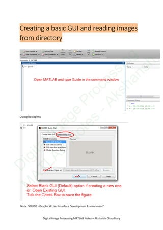
Converts Matrix to Grayscale image.
LOG
Note:
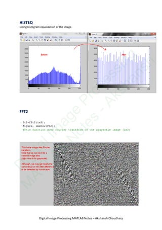
We saw that the frequency domain transform gave the results as black and white of my image. So,
we use logarithmic transform.
Applying log transformation to an image will expand its low valued pixels to a higher level and has
little effect on higher valued pixels so in other words it enhances image in such a way that it
highlights minor details of an image.
Commands:
a=imread('ATT00027.jpg');
a=im2double(a);
x=a;
[r,c]=size(a);
C=4;
for i=1:r
for j=1:c
D
igitalIm
age
Processing
M
ATLAB
N
otes
-Akshansh

x(i,j)=C*log(1+a(i,j));
end
end
subplot(1,2,1)
imshow(a);
title('Before Transformation');
subplot(1,2,2);
imshow(x);
title('After Transformation');
IFFT2, UINT8
IFFT2 command is used to do the inverse Fourier transform of the image.
UINT8 command is used to convert the image to an 8 bit signed integer.
D
igitalIm
age
Processing
M
ATLAB
N
otes
-Akshansh

ROT90
Note: Image rotation can only be done to 2D image.
That is, we can use it only for grayscale images.
D
igitalIm
age
Processing
M
ATLAB
N
otes
-Akshansh

Creating a basic GUI and reading images
from directory
Dialog box opens
Note: "GUIDE - Graphical User Interface Development Environment"
D
igitalIm
age
Processing
M
ATLAB
N
otes
-Akshansh

This opens a new GUI dialog box as shown -
D
igitalIm
age
Processing
M
ATLAB
N
otes
-Akshansh

Let's say we make a List Box.
As I aim to load the image, I have to put the images in the MATLAB Directory so that the images can
be accessed from there directly while coding is done.
D
igitalIm
age
Processing
M
ATLAB
N
otes
-Akshansh

In the GUI window, there is an AXES option.
Let's make two AXIS. One for the original image and other for the changed image.
Beautifying it, Put a panel first and then put Axes over it as shown.
D
igitalIm
age
Processing
M
ATLAB
N
otes
-Akshansh

Double click on Pop up menu opens Property Inspector window.
D
igitalIm
age
Processing
M
ATLAB
N
otes
-Akshansh

Creating a text file -
Open Notepad and write the names of all the file names in your current directory.
See that the names in the current directory (without the extension like .jpeg) are being copy pasted
in the Notepad.
Then, save the notepad file in the same MATLAB Directory
(By default, its C:UsersAkshanshDocumentsMATLAB)
D
igitalIm
age
Processing
M
ATLAB
N
otes
-Akshansh

D
igitalIm
age
Processing
M
ATLAB
N
otes
-Akshansh

Now,
We can also click on the properties and change the colors of the background and its title, etc.
As we save this program, it creates an m file.
D
igitalIm
age
Processing
M
ATLAB
N
otes
-Akshansh

We need to remove the values
Go back to figure window.
Double click on AXES. A dialog box opens.
D
igitalIm
age
Processing
M
ATLAB
N
otes
-Akshansh

Similarly do for Y axes.
Save the GUI and open m file
Run it.
All boundaries gone.
Now, make a duplicate of the (Axes+Panel).
One will be input, other will be output.
D
igitalIm
age
Processing
M
ATLAB
N
otes
-Akshansh

Add a push button
Change its properties if needed.
D
igitalIm
age
Processing
M
ATLAB
N
otes
-Akshansh

Save it and Run it.
Select image and press process.
Nothing happens, as, there is no code written for my GUI.
D
igitalIm
age
Processing
M
ATLAB
N
otes
-Akshansh

BITS PILANI DUBAI CAMPUS
MATLAB ASSIGNMENT QUESTIONS FOR DIGITAL IMAGE PROCESSING AND IMAGE
PROCESSING
Note: ANY FIVE out of six questions have to be implemented in MATLAB.
Hand written sheets of program codes have to be submitted (not the soft copy).
Question 1.
Write a MATLAB based GUI program, to illustrate the power law transformation
Question 2.
Write a MATLAB based GUI program, to illustrate intensity level slicing and bit level slicing
Question 3.
Write a MATLAB based GUI program to illustrate Steganography.
Question 4.
Write a GUI based MATLAB program to detect the boundary of the object using Hough transform.
Question 5.
Write a MATLAB based GUI program to illustrate removal of periodic noise from an image using a Notch Filter
(Band Stop Filter).
Question 6.
Write a MATLAB based GUI program to illustrate the effect of Atmospheric Turbulence on an image and how the
image can be retrieved from the noise.
Lecture Notes
D
igitalIm
age
Processing
M
ATLAB
N
otes
-Akshansh

DIP (EEE F435)
MATLAB Assignment Program
1 POWER LAW TRANSFORMATION
unction varargout = Gamma_Transform(varargin)
% GAMMA_TRANSFORM MATLAB code for Gamma_Transform.fig
% GAMMA_TRANSFORM, by itself, creates a new GAMMA_TRANSFORM or raises
the existing
% singleton*.
%
% H = GAMMA_TRANSFORM returns the handle to a new GAMMA_TRANSFORM or the
handle to
% the existing singleton*.
%
% GAMMA_TRANSFORM('CALLBACK',hObject,eventData,handles,...) calls the
local
% function named CALLBACK in GAMMA_TRANSFORM.M with the given input
arguments.
%
% GAMMA_TRANSFORM('Property','Value',...) creates a new GAMMA_TRANSFORM
or raises the
% existing singleton*. Starting from the left, property value pairs are
% applied to the GUI before Gamma_Transform_OpeningFcn gets called. An
% unrecognized property name or invalid value makes property application
% stop. All inputs are passed to Gamma_Transform_OpeningFcn via
varargin.
%
% *See GUI Options on GUIDE's Tools menu. Choose "GUI allows only one
% instance to run (singleton)".
%
% See also: GUIDE, GUIDATA, GUIHANDLES
% Edit the above text to modify the response to help Gamma_Transform
% Last Modified by GUIDE v2.5 14-May-2014 22:44:13
% Begin initialization code - DO NOT EDIT
gui_Singleton = 1;
gui_State = struct('gui_Name', mfilename, ...
'gui_Singleton', gui_Singleton, ...
'gui_OpeningFcn', @Gamma_Transform_OpeningFcn, ...
'gui_OutputFcn', @Gamma_Transform_OutputFcn, ...
'gui_LayoutFcn', [] , ...
'gui_Callback', []);
if nargin && ischar(varargin{1})
gui_State.gui_Callback = str2func(varargin{1});
end
if nargout
D
igitalIm
age
Processing
M
ATLAB
N
otes
-Akshansh

[varargout{1:nargout}] = gui_mainfcn(gui_State, varargin{:});
else
gui_mainfcn(gui_State, varargin{:});
end
% End initialization code - DO NOT EDIT
% --- Executes just before Gamma_Transform is made visible.
function Gamma_Transform_OpeningFcn(hObject, eventdata, handles, varargin)
% This function has no output args, see OutputFcn.
% hObject handle to figure
% eventdata reserved - to be defined in a future version of MATLAB
% handles structure with handles and user data (see GUIDATA)
% varargin command line arguments to Gamma_Transform (see VARARGIN)
% Choose default command line output for Gamma_Transform
handles.output = hObject;
% Update handles structure
guidata(hObject, handles);
% UIWAIT makes Gamma_Transform wait for user response (see UIRESUME)
% uiwait(handles.figure1);
% --- Outputs from this function are returned to the command line.
function varargout = Gamma_Transform_OutputFcn(hObject, eventdata, handles)
% varargout cell array for returning output args (see VARARGOUT);
% Get default command line output from handles structure
varargout{1} = handles.output;
% --- Executes on selection change in listbox1.
function listbox1_Callback(hObject, eventdata, handles)
% hObject handle to listbox1 (see GCBO)
% Hints: contents = cellstr(get(hObject,'String')) returns listbox1 contents
as cell array
% contents{get(hObject,'Value')} returns selected item from listbox1
global im;
contents = cellstr(get(hObject,'String'));
im=contents{get(hObject,'Value')};
im=strcat(im,'.jpg');
im=imread(im);
axes(handles.axes1);
imshow(im);
D
igitalIm
age
Processing
M
ATLAB
N
otes
-Akshansh

% --- Executes during object creation, after setting all properties.
function listbox1_CreateFcn(hObject, eventdata, handles)
% handles empty - handles not created until after all CreateFcns called
% Hint: listbox controls usually have a white background on Windows.
% See ISPC and COMPUTER.
if ispc && isequal(get(hObject,'BackgroundColor'),
get(0,'defaultUicontrolBackgroundColor'))
set(hObject,'BackgroundColor','white');
end
function edit1_Callback(hObject, eventdata, handles)
% hObject handle to edit1 (see GCBO)
% Hints: get(hObject,'String') returns contents of edit1 as text
% str2double(get(hObject,'String')) returns contents of edit1 as a
double
global cval;
% cval=get(hObject,'String');
cval=str2double(get(hObject,'String'));
function edit1_CreateFcn(hObject, eventdata, handles)
% Hint: edit controls usually have a white background on Windows.
end
% --- Executes on button press in pushbutton1.
function pushbutton1_Callback(hObject, eventdata, handles)
% hObject handle to pushbutton1 (see GCBO)
D
igitalIm
age
Processing
M
ATLAB
N
otes
-Akshansh

global im;
global im2;
im=rgb2gray(im);
im2=im2double(im);
imshow(im);
double
global gval;
% gval=get(hObject,'Value')
gval=str2double(get(hObject,'String'));
end
global im2;
global im3;
global cval;
global gval;
[m,n]=size(im2);
for i=1:m
D
igitalIm
age
Processing
M
ATLAB
N
otes
-Akshansh

for j=1:n
im3(i,j)=cval*((im2(i,j)/255).^gval);
end
end
imshow(im3);
2
2.1 INTENSITY LEVEL SLICING
function varargout = Intensity_Level_Slicing(varargin)
% INTENSITY_LEVEL_SLICING MATLAB code for Intensity_Level_Slicing.fig
% INTENSITY_LEVEL_SLICING, by itself, creates a new
INTENSITY_LEVEL_SLICING or raises the existing
% singleton*.
%
% H = INTENSITY_LEVEL_SLICING returns the handle to a new
INTENSITY_LEVEL_SLICING or the handle to
%
% INTENSITY_LEVEL_SLICING('CALLBACK',hObject,eventData,handles,...)
calls the local
% function named CALLBACK in INTENSITY_LEVEL_SLICING.M with the given
input arguments.
%
% INTENSITY_LEVEL_SLICING('Property','Value',...) creates a new
INTENSITY_LEVEL_SLICING or raises the
% applied to the GUI before Intensity_Level_Slicing_OpeningFcn gets
called. An
% stop. All inputs are passed to Intensity_Level_Slicing_OpeningFcn via
varargin.
%
%
% Edit the above text to modify the response to help Intensity_Level_Slicing
gui_Singleton = 1;
D
igitalIm
age
Processing
M
ATLAB
N
otes
-Akshansh

'gui_OpeningFcn', @Intensity_Level_Slicing_OpeningFcn, ...
'gui_OutputFcn', @Intensity_Level_Slicing_OutputFcn, ...
end
if nargout
else
end
% --- Executes just before Intensity_Level_Slicing is made visible.
function Intensity_Level_Slicing_OpeningFcn(hObject, eventdata, handles,
varargin)
% varargin command line arguments to Intensity_Level_Slicing (see VARARGIN)
% Choose default command line output for Intensity_Level_Slicing
% UIWAIT makes Intensity_Level_Slicing wait for user response (see UIRESUME)
function varargout = Intensity_Level_Slicing_OutputFcn(hObject, eventdata,
handles)
D
igitalIm
age
Processing
M
ATLAB
N
otes
-Akshansh

as cell array
global im1;
global im2;
global con;
con = cellstr(get(hObject,'String'));
im1=con{get(hObject,'Value')};
im1=strcat(im1, '.jpg');
im1=imread(im1);
im2=im1;
imshow(im1);
end
global im1;
global im2;
im2=rgb2gray(im1);
imshow(im2);
% --- Executes on slider movement.
function slider1_Callback(hObject, eventdata, handles)
% hObject handle to slider1 (see GCBO)
% Hints: get(hObject,'Value') returns position of slider
% get(hObject,'Min') and get(hObject,'Max') to determine range of
slider
D
igitalIm
age
Processing
M
ATLAB
N
otes
-Akshansh

global minval;
global maxval;
global tval;
tval=get(hObject,'Value');
if (tval>maxval || tval<minval)
msgbox(sprintf('Please choose Threshold value between Maximum and
Minimum'),'Error','Error');
return
end
data1 = strcat(num2str(tval));
set(handles.text1,'String',data1);
function slider1_CreateFcn(hObject, eventdata, handles)
% Hint: slider controls usually have a light gray background.
if isequal(get(hObject,'BackgroundColor'),
set(hObject,'BackgroundColor',[.9 .9 .9]);
end
slider
global maxval;
global minval;
minval=get(hObject,'Value');
if (minval>maxval)
msgbox(sprintf('Please choose Min. Value < Max Value'),'Error','Error');
return
end
data2 = strcat(num2str(minval));
D
igitalIm
age
Processing
M
ATLAB
N
otes
-Akshansh

end
slider
global minval;
global maxval;
maxval=get(hObject,'Value');
if (maxval<minval)
msgbox(sprintf('Please choose Max Value > Min Value'),'Error','Error');
return
end
data3 = strcat(num2str(maxval));
end
global tval;
global minval;
global maxval;
global im2;
[M,N]=size(im2);
if (minval<maxval)
for i=1:M
for j=1:N
if (im2(i,j)>tval)
im2(i,j)=maxval;
D
igitalIm
age
Processing
M
ATLAB
N
otes
-Akshansh

else
im2(i,j)=minval;
end
end
end
end
imshow(im2);
2.2 BIT PLANE SLICING
function varargout = Bit_Plane_Slicing(varargin)
% BIT_PLANE_SLICING MATLAB code for Bit_Plane_Slicing.fig
% BIT_PLANE_SLICING, by itself, creates a new BIT_PLANE_SLICING or
raises the existing
% singleton*.
%
% H = BIT_PLANE_SLICING returns the handle to a new BIT_PLANE_SLICING or
the handle to
%
% BIT_PLANE_SLICING('CALLBACK',hObject,eventData,handles,...) calls the
local
% function named CALLBACK in BIT_PLANE_SLICING.M with the given input
arguments.
%
% BIT_PLANE_SLICING('Property','Value',...) creates a new
BIT_PLANE_SLICING or raises the
% applied to the GUI before Bit_Plane_Slicing_OpeningFcn gets called.
An
% stop. All inputs are passed to Bit_Plane_Slicing_OpeningFcn via
varargin.
%
%
% Edit the above text to modify the response to help Bit_Plane_Slicing
gui_Singleton = 1;
'gui_OpeningFcn', @Bit_Plane_Slicing_OpeningFcn, ...
'gui_OutputFcn', @Bit_Plane_Slicing_OutputFcn, ...
D
igitalIm
age
Processing
M
ATLAB
N
otes
-Akshansh

end
if nargout
else
end
% --- Executes just before Bit_Plane_Slicing is made visible.
function Bit_Plane_Slicing_OpeningFcn(hObject, eventdata, handles, varargin)
% varargin command line arguments to Bit_Plane_Slicing (see VARARGIN)
% Choose default command line output for Bit_Plane_Slicing
% UIWAIT makes Bit_Plane_Slicing wait for user response (see UIRESUME)
function varargout = Bit_Plane_Slicing_OutputFcn(hObject, eventdata, handles)
as cell array
global im1;
im1= contents{get(hObject,'Value')};
im1=strcat(im1,'.jpg');
D
igitalIm
age
Processing
M
ATLAB
N
otes
-Akshansh

im1=imread(im1);
imshow(im1);
end
global im1;
global im2;
im2=rgb2gray(im1);
imshow(im2);
global im4;
global im2;
global bp1;
global bp2;
global bp3;
global bp4;
global bp5;
global bp6;
global bp7;
global bp8;
[m, n]=size(im2);
for i=1:m
for j=1:n
for k=1:8
if k==1
bp1(i,j)=bitget(im2(i,j),k);
else if k==2
D
igitalIm
age
Processing
M
ATLAB
N
otes
-Akshansh

else if k==3
else if k==4
else if k==5
else if k==6
else if k==7
else
end
end
end
end
end
end
end
end
end
end
imshow(bp1);
imshow(bp2);
imshow(bp3);
imshow(bp4);
imshow(bp5);
imshow(bp6);
imshow(bp7);
imshow(bp8);
for i=1:m
for j=1:n
im4(i,j)=bp1(i,j)/200+bp2(i,j)/200*2+bp3(i,j)/200*4+bp4(i,j)/200*8+bp5(i,j)/2
00*16+bp6(i,j)/200*32+bp7(i,j)/200*64+bp8(i,j)/200*128;
end
end
D
igitalIm
age
Processing
M
ATLAB
N
otes
-Akshansh

imshow(im4);
3 STEGANOGRAPHY
function varargout = Steganography(varargin)
% STEGANOGRAPHY MATLAB code for Steganography.fig
% STEGANOGRAPHY, by itself, creates a new STEGANOGRAPHY or raises the
existing
% singleton*.
%
% H = STEGANOGRAPHY returns the handle to a new STEGANOGRAPHY or the
handle to
%
% STEGANOGRAPHY('CALLBACK',hObject,eventData,handles,...) calls the
local
% function named CALLBACK in STEGANOGRAPHY.M with the given input
arguments.
%
% STEGANOGRAPHY('Property','Value',...) creates a new STEGANOGRAPHY or
raises the
% applied to the GUI before Steganography_OpeningFcn gets called. An
% stop. All inputs are passed to Steganography_OpeningFcn via varargin.
%
%
% Edit the above text to modify the response to help Steganography
gui_Singleton = 1;
'gui_OpeningFcn', @Steganography_OpeningFcn, ...
'gui_OutputFcn', @Steganography_OutputFcn, ...
end
if nargout
else
end
D
igitalIm
age
Processing
M
ATLAB
N
otes
-Akshansh

% --- Executes just before Steganography is made visible.
function Steganography_OpeningFcn(hObject, eventdata, handles, varargin)
% varargin command line arguments to Steganography (see VARARGIN)
% Choose default command line output for Steganography
% UIWAIT makes Steganography wait for user response (see UIRESUME)
function varargout = Steganography_OutputFcn(hObject, eventdata, handles)
as cell array
global im;
im=contents{get(hObject,'Value')};
im=strcat(im,'.jpg');
im=imread(im);
imshow(im);
D
igitalIm
age
Processing
M
ATLAB
N
otes
-Akshansh

end
global im;
im=rgb2gray(im);
imshow(im);
double
global txt;
global t2;
txt=get(hObject, 'String')
t2=de2bi(uint16(char(txt)))
end
D
igitalIm
age
Processing
M
ATLAB
N
otes
-Akshansh

global im;
global im2;
global bp1;
global t5;
global t6;
global t2;
global imx;
im2=im;
[m, n]=size(im2);
global n1;
global n2;
% n2=0;
for i=1:m
for j=1:n
bp1(i,j)=bitget(im2(i,j),1);
end
end
[t5, t6]=size(t2);
imx=zeros(t5,t6,8);
for i=1:t5
for j=1:t6
imx(i,j,1)=t2(i,j);
end
end
for i=1:t5
for j=1:t6
im2(i,j)=im2(i,j)-bp1(i,j)/200+bi2de(imx(i,j));
end
end
imshow(im2);
D
igitalIm
age
Processing
M
ATLAB
N
otes
-Akshansh

4 HOUGH TRANSFORM
%David Raedy
%Introduction to Computer vision and modeling
%Final Project -- Shape detection with Hough Transforms
%
%Hough transform is used to automatically detect
%features from an image that has has an edge detection
%algorithm applied.
%
%I have implemented two types of feature extraction:
%lines and circles, both of which involve transforming
%the image from "feature space" into "parameter space".
%The methods for extracting line and circle features
%are different enough to warrant separate explanations.
%
%Circle Extraction
%The more intuitive of the methods is circle extraction.
%It is more intuitive to me because the matrix representing
%the parameter space has the same dimensions as the original,
%and the method involves projecting circles using cartesian
%coordinates. Simply stated, each pixel in the edge-detected
%image serves as the centerpoint for a circle of a given radius.
%Circles are projected around the centerpoint, and for each point
%on the circle, the corresponding cell in the accumulator array
%is incremented by one.
%
%The result of projecting these circles of fixed array in the
%hough parameter space is that the centerpoints of circles in
%feature space is revealed: in parameter space those centerpoints
%will accumulate relatively large values, since the centerpoint
%will appear on the edge of all of the circles formed in
%parameter space by the edges of the actual circle in feature space.
%
%The drawback of this technique is that it is computationally
%complex, and requires separate passes for any give radius.
%It's also rigid, and only reveals nearly perfect circles.
%
%Line Extraction
%Line extraction operates in a similar vein, but is somewhat more
%abstract -- which is to say, you can view the accumulator matrix
%(parameter space) from circle extraction, and see pretty clearly
%how the process works, including being able to see vestiges of the
%original image. With line extraction, there is no such correlation:
%parameter space inhabits a different-sized matrix for one, and the
%axes represent minimum distance from the origin for a given line on
%the one hand, and angle of the line on the other.
%
%So the first thing to understand about parameter space for line
%extraction is that there is no one-to-one relationship between
%pixels in the image and cells in the parameter space matrix.
%Rather, each cell in parameter space represents a line that spans
%across the entire image.
%
%The transformation between feature space and parameter space is
%the following:
D
igitalIm
age
Processing
M
ATLAB
N
otes
-Akshansh

%Project a line through each edge pixel at every possible angle
%(you can also increment the angles at steps). For each line,
%calculate the minimum distance between the line and the origin.
%Increment the appropriate parameter space accumulator by one.
%The x-axis of parameter space ranges from 1 to the square root of
%the sum of the squares of rows and columns from feature space.
%(This number corresponds to the furthest possible minimum distance
%from the origin to a line passing through the image.
%The y-axis represents the angle of the line.
%Obviously the axes could be switched...
%
%Similarly to the process of circle extraction, the larger the number
%in any given cell of the accumulator matrix, the larger the likelihood
%that a line exists at that angle and distance from the origin.
%
%Transforming from parameter space back to feature space is slightly
%more trouble for lines than circles -- the method I employ involves
%the risk of divide-by-zero for one. Also, each line pixel is checked
%to see if there is a pixel in edge space, and marked accordingly.
%
%An extra step which I didn't employ would be to add a step of hysterisis
%to attempt to discover the line segments more definitively.
%
%The main trouble with both methods was finding an appropriate
%threshhold for determining what constitutes a feature. The image
%processing toolkit apparently has a local maximum detector, which
%would have been very helpful. I relied on a more blunt measure,
%which was a threshold as a percentage of the maximum accumulator
%value.
%
%----------------------------------------------
%canny edge detector section
%
%img=imread('parallelo.jpg');
img=imread('Amazing Scene in Burma.jpg');
%img=imread('scene_shapes_a.png');
F=(rgb2gray(img));
%display original image in grayscale
figure(1);
imagesc(F);
colormap(gray);
axis image;
% compute Gaussian
sig = 1.5;
x = floor(-3*sig):ceil(3*sig);
GAUSS = exp(-0.5*x.^2/sig^2);
GAUSS = GAUSS/sum(GAUSS);
dGAUSS = -x.*GAUSS/sig^2;
% convolute the image with kernel
Kx = GAUSS'*dGAUSS;
Ky = Kx';
D
igitalIm
age
Processing
M
ATLAB
N
otes
-Akshansh

Ix=conv2(F, Kx, 'same');
Iy=conv2(F, Ky, 'same');
%determine a range and scale for tossing out noise later
%(only look at relatively strong edges)
maxIx = max(max(Ix));
minIx = min(min(Ix));
scaleIx = (maxIx-minIx)/10.0;
maxIy = max(max(Iy));
minIy = min(min(Iy));
scaleIy = (maxIy-minIy)/10.0;
%threshhold is a little arbitrary
strThresh = (0.5*scaleIx)^2 + (0.5*scaleIy)^2;
%initialize matrices for edge image and edge strengths
[rows,cols] = size(F);
Edges = zeros(rows,cols);
%edges binary records 1 for edge pixel and 0 otherwise
%used in hough transform
EdgesBinary = zeros(rows,cols);
Strength = zeros(rows,cols);
%calculate edge strengths
Strength = Ix.^2 + Iy.^2;
%define thresholds for arctan results
% of Iy/Ix (to determine orientation)
pi = 22.0/7.0;
pi8 = pi/8;
pi2 = 4.0*pi8;
threepi8 = 3.0 * pi8;
%value holds arctan orientation value temporarily for each pixel
value = 0;
%skip outermost pixel to avoid out of bounds errors
for x = 2:rows-1
for y = 2:cols-1
%set the edge image pixels to white
Edges(x,y) = 255;
%only proceed with orientation and edge strength if the result will be
defined
%and if edge strength is above threshhold
if( abs(Ix(x,y)) > 0.001 & Strength(x,y) > strThresh )
%get orientation
value = atan( Iy(x,y) / Ix(x,y) );
D
igitalIm
age
Processing
M
ATLAB
N
otes
-Akshansh

%horizontal orientation
if (value <= pi8 & value >= -1.0*pi8)
if Strength(x,y) > Strength(x,y-1) & Strength(x,y) >
Strength(x,y+1)
Edges(x,y) = 0;
EdgesBinary(x,y) = 1;
end
%negative slope orientation
elseif value < threepi8 & value > 0.0
if Strength(x,y) > Strength(x-1, y-1) & Strength(x,y) >
Strength(x+1, y+1)
Edges(x,y) = 0;
end
%positive slope orientation
elseif value > -1.0*threepi8 & value < 0.0
if Strength(x,y) > Strength(x-1, y+1) & Strength(x,y) >
Strength(x+1, y-1)
Edges(x,y) = 0;
end
else
%vertical orientation
if Strength(x,y) > Strength(x-1,y) & Strength(x,y) >
Strength(x+1,y)
Edges(x,y) = 0;
end
end
end
end
end
%this figure will display the canny edge results
figure(2);
image(Edges);
colormap(gray);
axis image;
%-----------------------------------------------
%begin hough transform stage, starting with lines
%
%variables controlling granularity of line search
dist_step = 1;
angle_incr = 2;
%set up Accumulator matrix based on size of image
[rows, cols] = size(EdgesBinary);
p = 1 : dist_step : sqrt(rows^2 + cols^2);
theta_deg = 0 : angle_incr : 360-angle_incr;
Accumulator = zeros(length(p), length(theta_deg));
%get indices of all edge pixels
[y_ind x_ind] = find(EdgesBinary > 0);
D
igitalIm
age
Processing
M
ATLAB
N
otes
-Akshansh

%iterate through each pixel
for i = 1 : size(x_ind)
theta_ind = 0;
%iterate through each angle through pixel
for theta_rad = theta_deg*pi/180
theta_ind = theta_ind+1;
%determine min distance to line calculated from origin
roi = x_ind(i)*cos(theta_rad) + y_ind(i)*sin(theta_rad);
if roi >= 1 & roi <= p(end)
temp = abs(roi-p);
mintemp = min(temp);
rad_ind = find(temp == mintemp);
rad_ind = rad_ind(1);
%add 1 to accumulator for this point at this angle
%the result is a matrix of numbers of lines,
%described by angle, and the point at which the
%line is a minimum distance from the origin
%naturally this is not a 1 to 1 relationship
%between line segments in the original image
%and lines described in hough parameter space
Accumulator(rad_ind,theta_ind) = Accumulator(rad_ind,theta_ind)+1;
end
end
end
%set threshold as percentage of max
thresh = 0.5 *(max(max(Accumulator(:))));
% get indices of lines (in parameter space) above threshold
[radius angle] = find(Accumulator > thresh);
temp_acc = Accumulator - thresh;
hough_rad = [];
hough_angle = [];
%take indices of instances where Accumulator > thresh
%and create vectors of distances from origin and angle
%from origin of line normal
for i = 1:length(radius)
if temp_acc(radius(i), angle(i)) >= 0
hough_rad = [hough_rad; radius(i)];
hough_angle = [hough_angle; angle(i)];
end
end
%adjust distance and angle to account for quantization level
%(steps/increments) in searching for lines
hough_rad = hough_rad * dist_step;
hough_angle = (hough_angle * angle_incr) - angle_incr;
D
igitalIm
age
Processing
M
ATLAB
N
otes
-Akshansh

%-------------------------------------------------------
%visualize the parameter space for lines
%x-axis is distance from origin in feature space
%y-axis is angle of line
figure(3);
image(Accumulator);
colormap(gray);
axis image;
%this figure will display the lines and circles
figure(4);
image(Edges);
colormap(gray);
axis image;
hold on;
[rows,cols] = size(Edges);
%need to convert degrees to radians again!!
hough_angle = hough_angle*pi/180;
for z = 1 : size(hough_rad)
for y = 1 : rows
%handle divide by zero situations
%(sin 0) = 0
if hough_angle(z) == 0
x = hough_rad(z);
if Edges(y,round(x)) == 0
plot(round(x),y,'b+');
else
plot(x,y,'c-');
end
else
x = ( hough_rad(z) / cos( hough_angle(z) )) - ( y *
sin( hough_angle(z) )) / cos( hough_angle(z));
%make sure y is within image matrix dimensions
%so that it can be plotted (for example y=0.34
%will give an error
if round(x) > 0 & round(x) < cols
%plot a blue '+' where line intersects edge
plot(round(x),y,'b+');
else
plot(round(x),y,'g+');
end
end
end
end
%handle divide by zero (cos 90)=0
D
igitalIm
age
Processing
M
ATLAB
N
otes
-Akshansh

for x = 1 : cols
if hough_angle(z) == 90
y = hough_rad(z);
%plot a blue '+' where line intersects edge
plot(x,round(y),'b+');
else
plot(x,round(y),'c-');
end
end
end
end
%-----------------------------------------------------
%now go after circles
%rad describes the radius of the circle being matched
%(the radius of the template being imposed on the image)
for rad = 50:75
%avoid hundreds of duplicate calculations
rad_sq = rad^2;
%accumulator for circles
AccCircles = zeros(size(EdgesBinary));
%grab indices of edge points in image
[yIndex xIndex] = find(EdgesBinary > 0);
for i = 1 : length(xIndex)
left = xIndex(i)-rad;
right = xIndex(i)+rad;
%allow for circles off the edge
if (left<1)
left=1;
end
%and the other edge
if (right > size(EdgesBinary,2) )
right = size(EdgesBinary,2);
end
%by projecting a circle around the edge points
%for each edge point, and adding one to the
%accumulator for each calculated point on that circle
%the effect is that the center point of any circle
%will have a relatively large value in the accumulator
%
%here the circle formula is applied, where
%x_offset iterates over the center+- radius
%and y_offset is calculated:
%y_offset = center_y +- sqrt( radius^2 - (center_x - x_offset)^2
for x_circ = left : right
rhs = sqrt(rad_sq - ( xIndex(i)-x_circ )^2 );
D
igitalIm
age
Processing
M
ATLAB
N
otes
-Akshansh

y_circ_a = yIndex(i) - rhs;
y_circ_b = yIndex(i) + rhs;
y_circ_a = round(y_circ_a);
y_circ_b = round(y_circ_b);
if y_circ_a < size(EdgesBinary,1) & y_circ_a >= 1
AccCircles(y_circ_a, x_circ) = AccCircles(y_circ_a, x_circ)+1;
end
if y_circ_b < size(EdgesBinary,1) & y_circ_b >= 1
AccCircles(y_circ_b, x_circ) = AccCircles(y_circ_b, x_circ)+1;
end
end
end
%set threshold, arbitrarily
thresh = 0.9 * max(max(AccCircles(:)));
% get centers of circles above threshold
xcoord = [];
ycoord = [];
[y_center x_center] = find(AccCircles > thresh);
temp_acc = AccCircles - thresh;
%and add to x and y coordinate value arrays
for i = 1:length(x_center)
if temp_acc(y_center(i), x_center(i)) >= 0
xcoord = [xcoord; x_center(i)];
ycoord = [ycoord; y_center(i)];
end
end
%-------------------------------
theta = [0:1:2*pi+1];
[xsize,ysize] = size(xcoord);
%reconstruct circles from centerpoints
for n_circ = 1:xsize
plot(xcoord(n_circ), ycoord(n_circ), '*');
x = rad * sin(theta);
y = rad * cos(theta);
%do this to initialize xoff/yoff to right size...
xoff = x;
yoff = y;
%reset values to correct offset
xoff(:) = xcoord(n_circ);
yoff(:) = ycoord(n_circ);
plot(x+xoff, y+yoff, 'c');
D
igitalIm
age
Processing
M
ATLAB
N
otes
-Akshansh

end
end
%finally visualize parameter space of circles
figure(5);
image(AccCircles);
colormap(gray);
axis image;
5 PERIODIC NOISE REMOVAL: NOTCH FILTER
%%%%%%%%%%%%%%%%%%%%%%%%%%%%%%%%%%%%%%%%%%%%%%%%%%%%%%%%%%%%%%%
%% im: input image
%% FT: Fourier transform of original image
%% mask : mask used for band reject filtering
%% FT2 : Band pass filtered spectrum
%% output : Denoised image
%%
%% Author: Krishna Kumar
%% Date: 25 Mar 2014
%%
%%One of the applications of band reject filtering is for noise removal
%%in applications where the general location of the noise component in
%%the frequency domain is approximately known.
%%
%% This program denoise an image corrupted by periodic noise that can be
%% approximated as two-dimensional sinusoidal functions using a band
%% reject filters.
%%You can adjust the radius of the filter mask to apply for a different
%%image.
%%%%%%%%%%%%%%%%%%%%%%%%%%%%%%%%%%%%%%%%%%%%%%%%%%%%%%%%%%%%%%%
clc;
clear all;
close all;
im = imread('imagename.extension');
figure,imshow(im);
FT = fft2(double(im));
FT1 = fftshift(FT);%finding spectrum
imtool(abs(FT1),[]);
m = size(im,1);
n = size(im,2);
t = 0:pi/20:2*pi;
xc=(m+150)/2; % point around which we filter image
yc=(n-150)/2;
r=200; %Radium of circular region of interest(for BRF)
r1 = 40;
xcc = r*cos(t)+xc;
ycc = r*sin(t)+yc;
xcc1 = r1*cos(t)+xc;
D
igitalIm
age
Processing
M
ATLAB
N
otes
-Akshansh

ycc1 = r1*sin(t)+yc;
mask = poly2mask(double(xcc),double(ycc), m,n);
mask1 = poly2mask(double(xcc1),double(ycc1), m,n);%generating mask for
filtering
mask(mask1)=0;
FT2=FT1;
FT2(mask)=0;%cropping area or bandreject filtering
imtool(abs(FT2),[]);
output = ifft2(ifftshift(FT2));
imtool(output,[]);
D
igitalIm
age
Processing
M
ATLAB
N
otes
-Akshansh

Digital Image Processing - MATLAB Notes - Akshansh

Recommended

Recommended

More Related Content

What's hot

What's hot (20)

Similar to Digital Image Processing - MATLAB Notes - Akshansh

Similar to Digital Image Processing - MATLAB Notes - Akshansh (20)

More from Akshansh Chaudhary

More from Akshansh Chaudhary (20)

Recently uploaded

Recently uploaded (20)

Digital Image Processing - MATLAB Notes - Akshansh