Assignment # 1 Due: Wednesday, Jan 24, 2007
CS223B Introduction to Computer Vision, Winter 2007
Please email your answers to stavens@robotics.stanford.edu.
Written Assignment #1
1 Introduction to Vision Software
Real-world implementation is essential in computer vision. Vision algorithms are often implemented in
software using either MATLAB or Intel’s Open Computer Vision (OpenCV) library for C/C++. The purpose
of this section is to gain an initial familiarity with these two environments. We ask that you implement
the four vision algorithms below. To encourage breadth, two of the algorithms must be implemented in
OpenCV and the other two must be implemented in MATLAB. Your code must be clearly structured and
well-commented. If obtaining access to MATLAB is an issue for you, please email the course staff as soon
as possible.
FAQ: Use gray-scale images where each pixel has a single intensity on [0:255].
FAQ: It is up to you which algorithms you implement in OpenCV and which you implement in MAT-
LAB. Sometimes OpenCV will be a cleaner choice than MATLAB or vice-versa. This will not affect your
grade.
FAQ: To check your work, you are free to implement each algorithm in every environment.
1.1 The Log-Polar Transform
The log-polar transform is a simple operation that changes the coordinate system of an image from Cartesian
to log-polar. Log-polar coordinates have several interesting properties. First, when optical flow is computed
as the camera moves along the optical axis (as is common in robotics), the optical flow vectors are radial
from the image center. However, in log-polar coordinates, the flow vectors are vertical. This can make the
detection of moving objects more efficient computationally. Second, the log polar transform converts an
image to a form that is rotation and scale invariant. This can be very helpful for object detection. Finally,
the log-polar transform emulates how images appear on the back of the human retina. (The brain then
transforms the image to the Cartesian-like way we perceive it.)
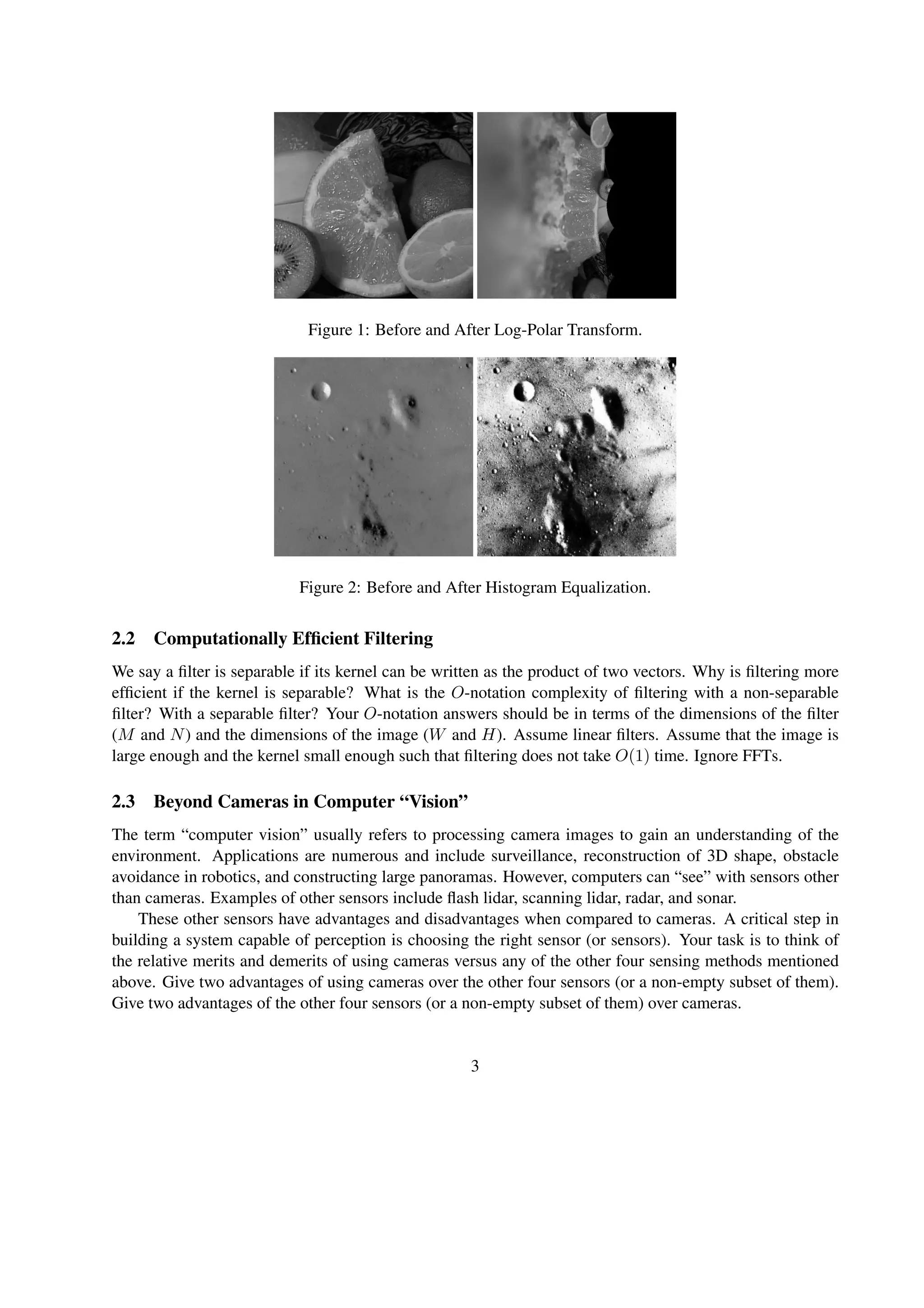
The log-polar transform is destination image[φ, ρ] = source image[x, y] where φ = tan−1(y/x) and
ρ = 60 ∗ loge x2 + y2. Leave any out-of-bounds pixels black.
Implement the transform on the image http://cs223b.stanford.edu/homework/ass1/1.1/input.png. Submit
your result as a PNG and the source code you used to generate it. An example of the log-polar transform
(on a different image) is included at the end of this document.
1.2 Background Subtraction
Tracking moving objects is an important problem in computer vision. When the camera is not moving, the
problem is often solvable if we know the background, that is, what the scene looks like when no moving
objects are present. Specifically, once the background is known, we can find moving objects by finding
regions of the current image that are different from the background image. (In practice, this approach is not
1
entirely successful since the background itself usually changes over time due to lighting, camera motion,
or other factors. Sophisticated algorithms exist for dealing with these problems. However, we ignore those
complexities for this assignment.)
We have put a sequence of images online at http://cs223b.stanford.edu/homework/ass1/1.2/. The images
are of the same scene. However, none is a background image since every image contains people in motion.
Using all the images together, extract the background image. (The solution is straightforward. No trickery
is needed.) Your program must use all of the images. You cannot manually select some subset of them.
Submit your result as a PNG and the source code you used to generate it.
1.3 Histogram Equalization
Often, we encounter an image whose dynamic range (ie: contrast) is compressed. For example, in an 8-bit
gray-scale image, only a narrow range of the 256 possible intensity values might be used. In that case, an
image can contain a significant amount of detail that is not apparent visually. One approach for enhancing
detail is called histogram equalization. It is straightforward to perform.
First, we generate a histogram H of the intensities in the image. Specifically, we have one bin for each
intensity 0-255. The value in each bin is the number of pixels in the image with that intensity. Second,
we normalize the histogram such that the sum of the 256 values in bins 0-255 is 255. Third, we generate a
second histogram H where H [i] = 0≤j≤i H[j] for all 0 ≤ i ≤ 255. Finally, destination image[x, y] =
H [source image[x, y]].
Implement the transform on the image http://cs223b.stanford.edu/homework/ass1/1.3/input.png. Submit
your result as a PNG and the source code you used to generate it. An example of histogram equalization (on
a different image) is at the end of this document.
FAQ: It is helpful to keep floating-point precision until you write the new image in the last step. Other-
wise, integer rounding will throw you off.
1.4 Contrast Stretching
Another approach to detail enhancement in the face of dynamic range compression (see Section 1.3) is
contrast stretching. Contrast stretching is even easier than histogram equalization:
destination image[x, y] = (source image[x, y] - image min) 255
image max - image min
where image min and image max are the minimum and maximum intensity values present in the image.
Implement the transform on the image http://cs223b.stanford.edu/homework/ass1/1.4/input.png. Submit
your result as a PNG and the source code you used to generate it.
2 Short Answer Questions
2.1 Orthographic and Perspective Projection
Let p and r be the endpoints of a line segment. Let q be some point on the segment. Let α = |q−r|
|q−p|. Is
α invariant under orthographic projection? What about perspective projection? For each question, if α is
invariant, prove it mathematically. If not, briefly explain.
2
Figure 1: Before and After Log-Polar Transform.
Figure 2: Before and After Histogram Equalization.
2.2 Computationally Efficient Filtering
We say a filter is separable if its kernel can be written as the product of two vectors. Why is filtering more
efficient if the kernel is separable? What is the O-notation complexity of filtering with a non-separable
filter? With a separable filter? Your O-notation answers should be in terms of the dimensions of the filter
(M and N) and the dimensions of the image (W and H). Assume linear filters. Assume that the image is
large enough and the kernel small enough such that filtering does not take O(1) time. Ignore FFTs.
2.3 Beyond Cameras in Computer “Vision”
The term “computer vision” usually refers to processing camera images to gain an understanding of the
environment. Applications are numerous and include surveillance, reconstruction of 3D shape, obstacle
avoidance in robotics, and constructing large panoramas. However, computers can “see” with sensors other
than cameras. Examples of other sensors include flash lidar, scanning lidar, radar, and sonar.
These other sensors have advantages and disadvantages when compared to cameras. A critical step in
building a system capable of perception is choosing the right sensor (or sensors). Your task is to think of
the relative merits and demerits of using cameras versus any of the other four sensing methods mentioned
above. Give two advantages of using cameras over the other four sensors (or a non-empty subset of them).
Give two advantages of the other four sensors (or a non-empty subset of them) over cameras.
3

Log polar coordinates

  • 1.
    Assignment # 1Due: Wednesday, Jan 24, 2007 CS223B Introduction to Computer Vision, Winter 2007 Please email your answers to stavens@robotics.stanford.edu. Written Assignment #1 1 Introduction to Vision Software Real-world implementation is essential in computer vision. Vision algorithms are often implemented in software using either MATLAB or Intel’s Open Computer Vision (OpenCV) library for C/C++. The purpose of this section is to gain an initial familiarity with these two environments. We ask that you implement the four vision algorithms below. To encourage breadth, two of the algorithms must be implemented in OpenCV and the other two must be implemented in MATLAB. Your code must be clearly structured and well-commented. If obtaining access to MATLAB is an issue for you, please email the course staff as soon as possible. FAQ: Use gray-scale images where each pixel has a single intensity on [0:255]. FAQ: It is up to you which algorithms you implement in OpenCV and which you implement in MAT- LAB. Sometimes OpenCV will be a cleaner choice than MATLAB or vice-versa. This will not affect your grade. FAQ: To check your work, you are free to implement each algorithm in every environment. 1.1 The Log-Polar Transform The log-polar transform is a simple operation that changes the coordinate system of an image from Cartesian to log-polar. Log-polar coordinates have several interesting properties. First, when optical flow is computed as the camera moves along the optical axis (as is common in robotics), the optical flow vectors are radial from the image center. However, in log-polar coordinates, the flow vectors are vertical. This can make the detection of moving objects more efficient computationally. Second, the log polar transform converts an image to a form that is rotation and scale invariant. This can be very helpful for object detection. Finally, the log-polar transform emulates how images appear on the back of the human retina. (The brain then transforms the image to the Cartesian-like way we perceive it.) The log-polar transform is destination image[φ, ρ] = source image[x, y] where φ = tan−1(y/x) and ρ = 60 ∗ loge x2 + y2. Leave any out-of-bounds pixels black. Implement the transform on the image http://cs223b.stanford.edu/homework/ass1/1.1/input.png. Submit your result as a PNG and the source code you used to generate it. An example of the log-polar transform (on a different image) is included at the end of this document. 1.2 Background Subtraction Tracking moving objects is an important problem in computer vision. When the camera is not moving, the problem is often solvable if we know the background, that is, what the scene looks like when no moving objects are present. Specifically, once the background is known, we can find moving objects by finding regions of the current image that are different from the background image. (In practice, this approach is not 1
  • 2.
    entirely successful sincethe background itself usually changes over time due to lighting, camera motion, or other factors. Sophisticated algorithms exist for dealing with these problems. However, we ignore those complexities for this assignment.) We have put a sequence of images online at http://cs223b.stanford.edu/homework/ass1/1.2/. The images are of the same scene. However, none is a background image since every image contains people in motion. Using all the images together, extract the background image. (The solution is straightforward. No trickery is needed.) Your program must use all of the images. You cannot manually select some subset of them. Submit your result as a PNG and the source code you used to generate it. 1.3 Histogram Equalization Often, we encounter an image whose dynamic range (ie: contrast) is compressed. For example, in an 8-bit gray-scale image, only a narrow range of the 256 possible intensity values might be used. In that case, an image can contain a significant amount of detail that is not apparent visually. One approach for enhancing detail is called histogram equalization. It is straightforward to perform. First, we generate a histogram H of the intensities in the image. Specifically, we have one bin for each intensity 0-255. The value in each bin is the number of pixels in the image with that intensity. Second, we normalize the histogram such that the sum of the 256 values in bins 0-255 is 255. Third, we generate a second histogram H where H [i] = 0≤j≤i H[j] for all 0 ≤ i ≤ 255. Finally, destination image[x, y] = H [source image[x, y]]. Implement the transform on the image http://cs223b.stanford.edu/homework/ass1/1.3/input.png. Submit your result as a PNG and the source code you used to generate it. An example of histogram equalization (on a different image) is at the end of this document. FAQ: It is helpful to keep floating-point precision until you write the new image in the last step. Other- wise, integer rounding will throw you off. 1.4 Contrast Stretching Another approach to detail enhancement in the face of dynamic range compression (see Section 1.3) is contrast stretching. Contrast stretching is even easier than histogram equalization: destination image[x, y] = (source image[x, y] - image min) 255 image max - image min where image min and image max are the minimum and maximum intensity values present in the image. Implement the transform on the image http://cs223b.stanford.edu/homework/ass1/1.4/input.png. Submit your result as a PNG and the source code you used to generate it. 2 Short Answer Questions 2.1 Orthographic and Perspective Projection Let p and r be the endpoints of a line segment. Let q be some point on the segment. Let α = |q−r| |q−p|. Is α invariant under orthographic projection? What about perspective projection? For each question, if α is invariant, prove it mathematically. If not, briefly explain. 2
  • 3.
    Figure 1: Beforeand After Log-Polar Transform. Figure 2: Before and After Histogram Equalization. 2.2 Computationally Efficient Filtering We say a filter is separable if its kernel can be written as the product of two vectors. Why is filtering more efficient if the kernel is separable? What is the O-notation complexity of filtering with a non-separable filter? With a separable filter? Your O-notation answers should be in terms of the dimensions of the filter (M and N) and the dimensions of the image (W and H). Assume linear filters. Assume that the image is large enough and the kernel small enough such that filtering does not take O(1) time. Ignore FFTs. 2.3 Beyond Cameras in Computer “Vision” The term “computer vision” usually refers to processing camera images to gain an understanding of the environment. Applications are numerous and include surveillance, reconstruction of 3D shape, obstacle avoidance in robotics, and constructing large panoramas. However, computers can “see” with sensors other than cameras. Examples of other sensors include flash lidar, scanning lidar, radar, and sonar. These other sensors have advantages and disadvantages when compared to cameras. A critical step in building a system capable of perception is choosing the right sensor (or sensors). Your task is to think of the relative merits and demerits of using cameras versus any of the other four sensing methods mentioned above. Give two advantages of using cameras over the other four sensors (or a non-empty subset of them). Give two advantages of the other four sensors (or a non-empty subset of them) over cameras. 3