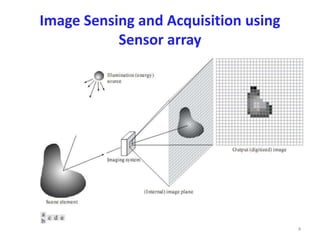
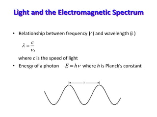
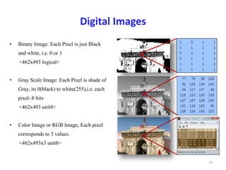
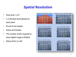
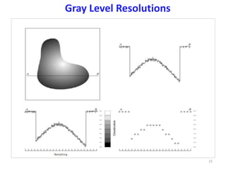
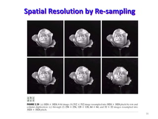
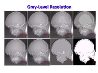
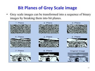
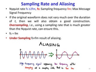
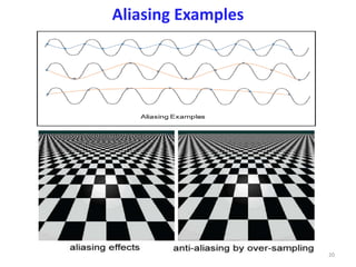
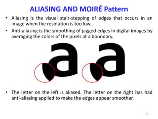
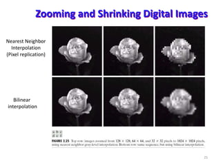
This document provides an overview of digital image fundamentals including: - The electromagnetic spectrum and how light is sensed and sampled by sensor arrays to create digital images. - Common sensor technologies like CCD and CMOS sensors and how they work. - How digital images are represented through spatial and intensity discretization via sampling and quantization. - Factors that affect image quality like spatial and intensity resolution. - Concepts like aliasing, moire patterns, and their relationship to sampling rates. - Basic image processing techniques like zooming, shrinking, and relationships between pixels.

1. Digital Image Fundamentals
Kalyan Acharjya
kalyan5.blogspot.in
Lecture 6-7
Unit 2
1

2. Unit 2
• Image Perception in Eye
• Light and Electromagnetic Spectrum
• Image Sensing and Acquisition using Sensor array.
• Image Sampling and Quantization
• Representation of Digital Image
• Spatial and Grey Level Resolutions
• Alising and Moire Pattern
• Zooming and Shrinking Digital Image
• Relationship Between Pixels
2

3. Disclaimer
This PPT is prepared for Academic use only.
Most of the Images and Contents are copied
from Image Processing Book (Gonzalez) and
Internet.
3

4. Image Sensing and Acquisition using
Sensor array
4

5. Light and the Electromagnetic Spectrum
• Relationship between frequency ( ) and wavelength ( )
,
where c is the speed of light
• Energy of a photon where h is Planck’s constant



c

hE 

6. Light and the Electromagnetic Spectrum
• Three basic quantities described the quality of
a chromatic light source:
– Radiance: the total amount energy that flow from
the light source (can be measured)
– Luminance: the amount of energy an observer
perceives from a light source (can be measured)
– Brightness: A subjective descriptor of light
perception; perceived quantity of light emitted
(cannot be measured)
6

7. CCD and CMOS Sensors?
• Array of Diodes (photo-diodes) that produce a
voltage:
– Linearly Proportional to the AMOUNT incident light.
– Non-linearly Dependant to the WAVELENGTH
• Built out of layers of Silicon
– Silicone is sensitive to light
– Layers add functionality–different layers perform different
functions. (called ‘die’)
7

8. CCD vs. CMOS
• Create high-quality, low-
noise images.
• Greater sensitivity and
fidelity
• 100 times more power
Require
• Specialized assembly lines
• Older and more developed
technology
• More susceptible to
noise
• Light sensitivity is lower
• Consume little power
• Easy to Manufacture
• Cheaper
Picture quality, sensitivity and cost vs. Cost and battery life.
8

9. Types of CCD and CMOS
CCD and CMOS
Rotational Lens
• Cheaper
• Good quality
• 3 frames req’d – only
stationary objects
Filter Array
• Cheap
• Easy
• Small
Beam Splitters
• Expensive
• High Quality
• One frame
required
Sony’s FS700, F5 and F55 cameras all have 4K sensors.
9

10. Sampling–Analog Signal
• Periodic sampling, the process of representing a
continuous signal with a sequence of discrete data values,
uses in the field of digital signal processing.
• In practice, sampling is performed by applying a
continuous signal to an analog-to-digital (A/D) converter
whose output is a series of digital values.
• With regard to sampling, the primary concern is how fast
must the given continuous signal be sampled in order to
preserve its information content.
10

11. Representation of a Digital Image
• An Image has infinite intensity value.
• Also infinite picture point .
• Digitization of image.
 Spatial discretization by Sampling.
 Intensity discretization by Quantization.
11

12. Representation of a Digital Image
12

13. Digital Images
• Binary Image: Each Pixel is just Black
and white, i.e. 0 or 1
<462x493 logical>
• Gray Scale Image: Each Pixel is shade of
Gray, its 0(black) to white(255),i.e. each
pixel~8 bits
<462x493 unit8>
• Color Image or RGB Image, Each pixel
corresponds to 3 values.
<462x493x3 unit8>
13

14. Spatial Resolution
• Gray level L=2k
• L is discrete level allowed to
each pixel.
• M and N are spatial
• Halve and Double
• The number of bits required to
store digital image b=MxNxk
• When M=N, b= kN2
14

15. Gray Level Resolutions
15

16. Spatial Resolution by Re-sampling
16

17. Gray-Level Resolution
24
816128
3264
256
17

18. Bit Planes of Grey Scale image
• Grey scale images can be transformed into a sequence of binary
images by breaking them into bit planes.
18

19. Sampling Rate and Aliasing
• Nyquist rate fs ≥2fm, fs: Sampling frequency fm: Max Message
Signal Frequency
• If the original waveform does not vary much over the duration
of t, then we will also obtain a good construction.
Oversampling, i.e., using a sampling rate that is much greater
than the Nyquist rate, can ensure this.
• fs = fm
• Under Sampling fs<fm result of aliasing.
19

20. Aliasing Examples
20

21. Aliasing and Moiré Pattern
• All signals (functions) can be shown to be made up of a linear
combination sinusoidal signals (sines and cosines) of different
frequencies. (Chapter 4)
• For physical reasons, there is a highest frequency component
in all real world signals.
• Theoretically,
– if a signal is sampled at more than twice its highest frequency
component, then it can be reconstructed exactly from its samples.
– But, if it is sampled at less than that frequency (called under sampling),
then aliasing will result.
– This causes frequencies to appear in the sampled signal that were not
in the original signal.
– The Moiré pattern shown the vertical low frequency pattern is a new
frequency not in the original patterns.
21

22. Moiré Pattern
22

23. ALIASING AND MOIRÉ Pattern
• Aliasing is the visual stair-stepping of edges that occurs in an
image when the resolution is too low.
• Anti-aliasing is the smoothing of jagged edges in digital images by
averaging the colors of the pixels at a boundary.
• The letter on the left is aliased. The letter on the right has had
anti-aliasing applied to make the edges appear smoother.
23

24. Zooming and Shrinking Digital Images
• Zooming: Increasing the number of pixels in
an image so that the image appears larger
– Nearest Neighbor Interpolation
• For example: pixel replication--to repeat rows and
columns of an image
– Bilinear interpolation
• Smoother
– Higher order interpolation
• Image shrinking: Sub-sampling
24

25. Zooming and Shrinking Digital Images
Nearest Neighbor
Interpolation
(Pixel replication)
Bilinear
interpolation
25

26. Some Basic Relationships Between Pixels
 Neighbors of a Pixel
There are three kinds of neighbors of a pixel-
• N4(p) 4-neighbors: the set of horizontal and vertical neighbors
• ND(p) diagonal neighbors: the set of 4 diagonal neighbors
• N8(p) 8-neighbors: union of 4-neighbors and diagonal neighbors
O O O
O X O
O O O
O O
X
O O
O
O X O
O

27. Some Basic Relationships Between Pixels
 Adjacency:
– Two pixels that are neighbors and have the same grey-level
(or some other specified similarity criterion) are adjacent
– Pixels can be 4-adjacent, diagonally adjacent, 8-adjacent, or
m-adjacent.
 m-adjacency (mixed adjacency):
– Two pixels p and q of the same value (or specified similarity)
are m-adjacent if either
• (i) q and p are 4-adjacent, or
• (ii) p and q are diagonally adjacent and do not have any common 4-
adjacent neighbors.
• They cannot be both (i) and (ii).

28. Some Basic Relationships Between Pixels
• An example of adjacency:
28

29. Some Basic Relationships Between Pixels
• Distance Measures
– Distance function: a function of two points, p and q, in
space that satisfies three criteria
– The Euclidean distance De(p, q)
),,(),()(
0),()(
pqDqpDb
qpDa


22
)()(),( tysxqpDe 

30. Hello 7CS
Your Choice!
30

31. Internal Marks Distribution
31
Maximum Marks Your Score (MM:30)
Mid Term I 20 x1
Mid Term I 20 x2
Test 10 x3
Attendance 10 x4
Total=60
Internal Score: (x1+x2+x3+x4)/2 (Minimum)

32. Thank You for
Your Attention
This PPT is available at kalyan5.blogspot.in
For Feedback Kindly visit
https://goo.gl/iPviBm
Contact E-mail: kalyan.acharjya@gmail.com
Good Luck
For Your
Mid Term I Examination
32