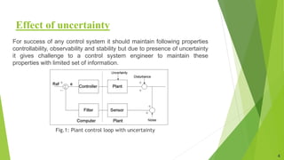
The document presents an overview of a dissertation preliminary presentation on the robustness characteristics of controllers and IMC-based controllers. It discusses topics like the effect of uncertainty, robust control toolbox algorithms, robustness analysis of controllers, internal model control, IMC-based controller design for delay-free and time-delay processes, tuning IMC-based PID controllers, and comparing the performance of traditional controllers to IMC-based controllers. Examples are provided to illustrate IMC-based controller design and tuning for first-order and second-order systems. Simulation results show IMC controllers achieve better rise time, settling time and overshoot compared to auto-tuned controllers.


![Procedure to find Controller Parameter
TSmith(s) = [Gc(s)Gm(s)e−Lm s] / [1 + Gc(s)Gm(s)]………(1)
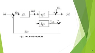
The closed-loop transfer function of the IMC design, assuming
a perfect matching and d = 0.
TIMC(s) = GIMC(s)G(s)…………(2)
TIMC(s) = GIMC(s)Gm(s) e−Ls …….(3)
From Eq.(1) and Eq.(3)
G(s) = Gc(s)/[1 + Gc(s)Gm(s)]…….(4)
Gc(s) = GIMC(s) / [1 − GIMC(s)Gm(s)]……….(5)
27](https://image.slidesharecdn.com/dissertationankitppt-240416052218-cc18c88f/85/Design-of-imc-based-controller-for-industrial-purpose-27-320.jpg)