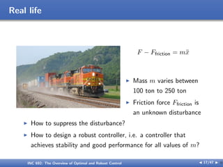
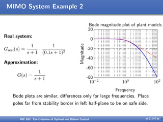
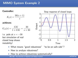
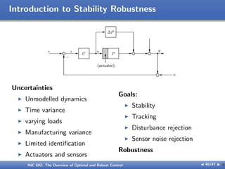
The document outlines the principles of optimal and robust control, detailing systematic design processes that include modeling, analysis, controller design, and implementation. It discusses classical and modern control theories, presents examples like space shuttle reentry and hard disk drive control, and emphasizes the importance of addressing uncertainties in system parameters. The text also highlights the significance of robust controllers in ensuring stability and performance amidst various disturbances and uncertainties.
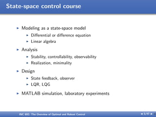
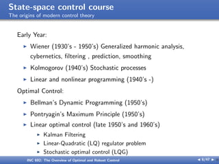


![ACC Benchmark problem
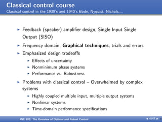
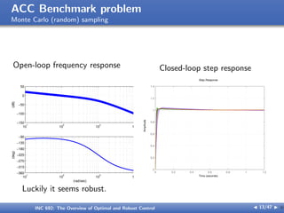
Monte Carlo (random) sampling
I New assumption
I Mass and spring constant are uncertain
k, m1, m2 ∈ [0.8, 1.2]
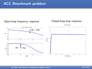
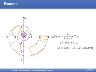
P(s) =
k
s2(m1m2s2 + k(m1 + m2))
I For perturbations of these parameters, how will the CL
stability and performance change?
INC 692: The Overview of Optimal and Robust Control J 12/47 I }](https://image.slidesharecdn.com/lecture02014-240424073907-1800b8ce/85/The-Overview-of-Optimal-and-Robust-Control-12-320.jpg)
![ACC Benchmark problem
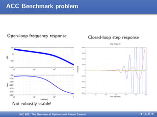
I New assumption
I Mass and spring constant are uncertain
k = 6 ± 20%, m1, m2 ∈ [0.8, 1.2]
P(s) =
k
s2(m1m2s2 + k(m1 + m2))
I For perturbations of these parameters, how will the CL
stability and performance change?
INC 692: The Overview of Optimal and Robust Control J 14/47 I }](https://image.slidesharecdn.com/lecture02014-240424073907-1800b8ce/85/The-Overview-of-Optimal-and-Robust-Control-14-320.jpg)
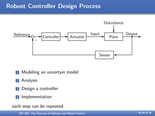
![MIMO System Example
Consider a multi-input/multi-output (MIMO) system:
[
Y1(s)
Y2(s)
]
= G(s)
[
U1(s)
U2(s)
]
with G(s) =
[
1
s+1
4
s+8
0.5
s+1
1
s+1
]
Suppose we neglect off-diagonal terms and choose the control
structure
U1(s) = K1(s)(R1(s) − Y1(s)) and U2(s) = K2(s)(R2(s) − Y2(s)), i.e.,
[
U1(s)
U2(s)
]
= K(s)
[
R1(s) − Y1(s)
R2(s) − Y2(s)
]
with K(s) =
[
K1(s) 0
0 K2(s)
]
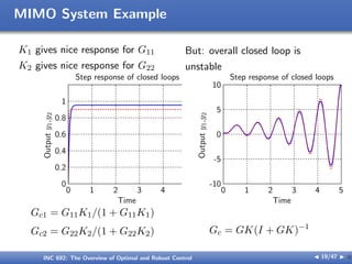
with K1(s) = 20 and K2(s) = 18.
INC 692: The Overview of Optimal and Robust Control J 18/47 I }](https://image.slidesharecdn.com/lecture02014-240424073907-1800b8ce/85/The-Overview-of-Optimal-and-Robust-Control-18-320.jpg)
![MIMO System Example
Why is the closed loop unstable?
ans: G has zero in right half-plane, and controllers gains are too
big
G(s) =
[
1
s+1
4
s+8
0.5
s+1
1
s+1
]
I How can we determine properties of MIMO systems?
I How should we design MIMO controllers for MIMO plants?
INC 692: The Overview of Optimal and Robust Control J 20/47 I }](https://image.slidesharecdn.com/lecture02014-240424073907-1800b8ce/85/The-Overview-of-Optimal-and-Robust-Control-20-320.jpg)
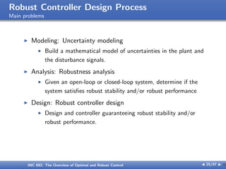
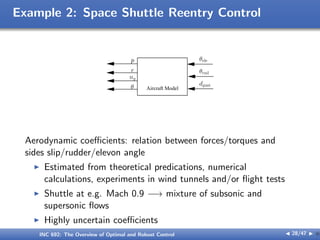
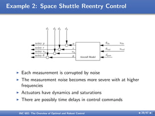
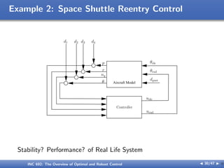
![Example 2: Space Shuttle Reentry Control
x =
β
p
r
ϕ
=
side slip angle
roll rate
yaw rate
bank angle
y =
p
r
ny
ϕ
, ny = lateral acceleration
u =
θele
θrud
dgust
=
elevon surface angle
rudder surface angle
lateral wind gusts
[1] Doyle, et al, “Design example using µ-synthesis: space shuttle lateral axis FCS
during reentry”, IEEE CDC, 1986
[2] Mu toolbox for MATLAB, user guide
INC 692: The Overview of Optimal and Robust Control J 27/47 I }](https://image.slidesharecdn.com/lecture02014-240424073907-1800b8ce/85/The-Overview-of-Optimal-and-Robust-Control-27-320.jpg)

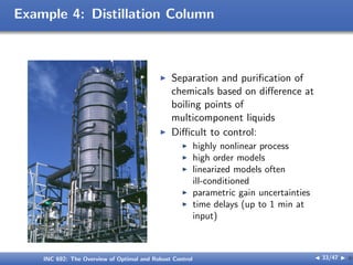
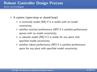
![Example 4: Distillation Column
[1 ] Skogestad, et al., Robust Control of ill-conditioned plants: high purity distillation, IEEE TAC, 1988
[2 ] Gu, Petkov, Konstantinov, Robust Control Design with MATLAB, Springer-Verlag, 2005
INC 692: The Overview of Optimal and Robust Control J 34/47 I }](https://image.slidesharecdn.com/lecture02014-240424073907-1800b8ce/85/The-Overview-of-Optimal-and-Robust-Control-34-320.jpg)
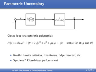
![Parametric Uncertainty
e k+Tds
1+T0s
u g
s2(1+θs)
y
−
G(s) =
g
s2(1 + sθ)
, g ∈ [g1, g2] , θ ∈ [θ1, θ2]
g = g0 +
g2 − g1
2
δg, g0 =
g1 + g2
2
, |δg| ≤ 1
θ = θ0 +
θ2 − θ1
2
δθ, θ0 =
θ1 + θ2
2
, |δθ| ≤ 1
Nominal system: G0(s) =
g0
s2(1 + sθ0)
A set of perturbed systems: G(s) =
g(δ)
s2(1 + sθ(δ))
INC 692: The Overview of Optimal and Robust Control J 37/47 I }](https://image.slidesharecdn.com/lecture02014-240424073907-1800b8ce/85/The-Overview-of-Optimal-and-Robust-Control-37-320.jpg)
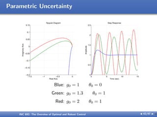
![Parametric Uncertainty
e k+Tds
1+T0s
u g
s2(1+θs)
y
−
I Nominal plat: g = g0 = 1, θ = 0
I Controller : k = 1, Td =
√
2, T0 = 1/10
I Perturbed plant: g ∈ [g, g], θ ∈ [0, θ]
INC 692: The Overview of Optimal and Robust Control J 41/47 I }](https://image.slidesharecdn.com/lecture02014-240424073907-1800b8ce/85/The-Overview-of-Optimal-and-Robust-Control-41-320.jpg)