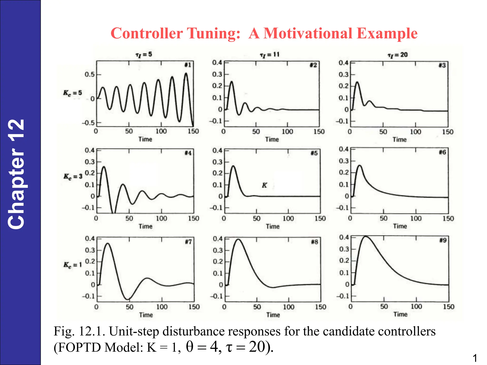
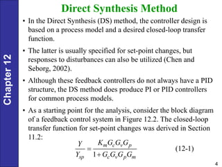
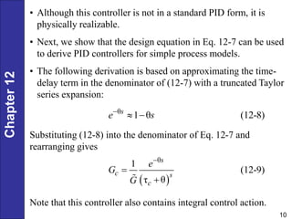
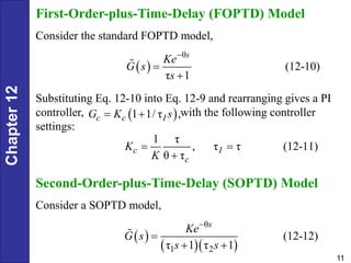
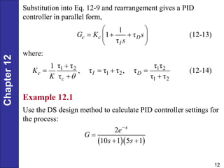
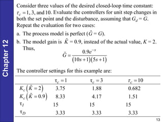
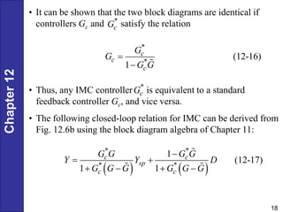
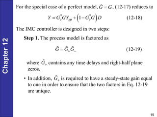
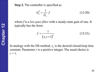
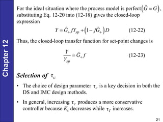
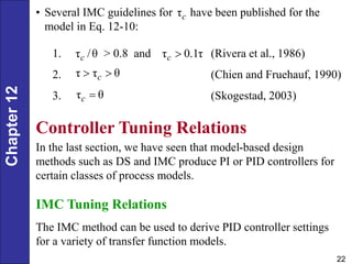
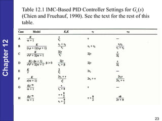
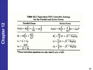
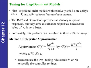
Chapter 12 discusses PID controller design, tuning, and performance criteria for closed-loop systems, emphasizing stability, disturbance rejection, and set-point tracking. It presents several tuning techniques, including direct synthesis and internal model control, detailing how to derive controller settings from process models. Additionally, the chapter illustrates the design of controllers for first-order and second-order systems, highlighting practical examples and modifications for lag-dominant models.

1. Chapter
12
1
Fig. 12.1. Unit-step disturbance responses for the candidate controllers
(FOPTD Model: K = 1, θ 4, τ 20).
 
Controller Tuning: A Motivational Example

2. Chapter
12
2
PID Controller Design, Tuning, and
Troubleshooting
Performance Criteria For Closed-Loop Systems
• The function of a feedback control system is to ensure that
the closed loop system has desirable dynamic and steady-
state response characteristics.
• Ideally, we would like the closed-loop system to satisfy the
following performance criteria:
1. The closed-loop system must be stable.
2. The effects of disturbances are minimized, providing
good disturbance rejection.
3. Rapid, smooth responses to set-point changes are
obtained, that is, good set-point tracking.

3. Chapter
12
3
4. Steady-state error (offset) is eliminated.
5. Excessive control action is avoided.
6. The control system is robust, that is, insensitive to
changes in process conditions and to inaccuracies in the
process model.
1. Direct Synthesis (DS) method
2. Internal Model Control (IMC) method
3. Controller tuning relations
4. Frequency response techniques
5. Computer simulation
6. On-line tuning after the control system is installed.
PID controller settings can be determined by a number
of alternative techniques:

4. Chapter
12
4
Direct Synthesis Method
• In the Direct Synthesis (DS) method, the controller design is
based on a process model and a desired closed-loop transfer
function.
• The latter is usually specified for set-point changes, but
responses to disturbances can also be utilized (Chen and
Seborg, 2002).
• Although these feedback controllers do not always have a PID
structure, the DS method does produce PI or PID controllers
for common process models.
• As a starting point for the analysis, consider the block diagram
of a feedback control system in Figure 12.2. The closed-loop
transfer function for set-point changes was derived in Section
11.2:
(12-1)
1
m c v p
sp c v p m
K G G G
Y
Y G G G G



5. Chapter
12
5
Fig. 12.2. Block diagram for a standard feedback control system.

6. Chapter
12
6
For simplicity, let and assume that Gm = Km. Then
Eq. 12-1 reduces to
v p m
G G G G
(12-2)
1
c
sp c
G G
Y
Y G G


Rearranging and solving for Gc gives an expression for the
feedback controller:
/
1
(12-3a)
1 /
sp
c
sp
Y Y
G
G Y Y
 
  
 

 
• Equation 12-3a cannot be used for controller design because the
closed-loop transfer function Y/Ysp is not known a priori.
• Also, it is useful to distinguish between the actual process G
and the model, , that provides an approximation of the
process behavior.
• A practical design equation can be derived by replacing the
unknown G by , and Y/Ysp by a desired closed-loop transfer
function, (Y/Ysp)d:
G
G

7. Chapter
12
7
 
 
/
1
(12-3b)
1 /
sp d
c
sp d
Y Y
G
G Y Y
 
 

 

 
• The specification of (Y/Ysp)d is the key design decision and will
be considered later in this section.
• Note that the controller transfer function in (12-3b) contains
the inverse of the process model owing to the term.
• This feature is a distinguishing characteristic of model-based
control.
1/G
Desired Closed-Loop Transfer Function
For processes without time delays, the first-order model in
Eq. 12-4 is a reasonable choice,
1
(12-4)
1
sp c
d
Y
Y s

 

 
  
 

8. Chapter
12
8
• The model has a settling time of ~ 4 , as shown in
Section 5. 2.
• Because the steady-state gain is one, no offset occurs for set-
point changes.
• By substituting (12-4) into (12-3b) and solving for Gc, the
controller design equation becomes:
τc
1 1
(12-5)
τ
c
c
G
s
G

• The term provides integral control action and thus
eliminates offset.
• Design parameter provides a convenient controller tuning
parameter that can be used to make the controller more
aggressive (small ) or less aggressive (large ).
1/ τcs
τc
τc
τc

9. Chapter
12
9
θ
(12-6)
τ 1
s
sp c
d
Y e
Y s

 

 
  
 
• If the process transfer function contains a known time delay ,
a reasonable choice for the desired closed-loop transfer
function is:
θ
• The time-delay term in (12-6) is essential because it is
physically impossible for the controlled variable to respond to
a set-point change at t = 0, before t = .
• If the time delay is unknown, must be replaced by an
estimate.
• Combining Eqs. 12-6 and 12-3b gives:
θ
θ
θ
θ
1
(12-7)
τ 1
s
c s
c
e
G
G s e



 

10. Chapter
12
10
• Although this controller is not in a standard PID form, it is
physically realizable.
• Next, we show that the design equation in Eq. 12-7 can be used
to derive PID controllers for simple process models.
• The following derivation is based on approximating the time-
delay term in the denominator of (12-7) with a truncated Taylor
series expansion:
θ
1 θ (12-8)
s
e s

 
Substituting (12-8) into the denominator of Eq. 12-7 and
rearranging gives
 
θ
1
(12-9)
τ θ



s
c s
c
e
G
G
Note that this controller also contains integral control action.

11. Chapter
12
11
First-Order-plus-Time-Delay (FOPTD) Model
Consider the standard FOPTD model,
 
θ
(12-10)
τ 1
s
Ke
G s
s



Substituting Eq. 12-10 into Eq. 12-9 and rearranging gives a PI
controller, with the following controller
settings:
 
1 1/ τ ,
c c I
G K s
 
1 τ
, τ τ (12-11)
θ τ
c I
c
K
K
 

Second-Order-plus-Time-Delay (SOPTD) Model
Consider a SOPTD model,
 
  
θ
1 2
(12-12)
τ 1 τ 1
s
Ke
G s
s s


 

12. Chapter
12
12
Substitution into Eq. 12-9 and rearrangement gives a PID
controller in parallel form,
1
1 τ (12-13)
τ
c c D
I
G K s
s
 
  
 
 
where:
1 2 1 2
1 2
1 2
τ τ τ τ
1
, τ τ τ , τ (12-14)
τ τ τ
c I D
c
K
K 

   
 
Example 12.1
Use the DS design method to calculate PID controller settings for
the process:
  
2
10 1 5 1
s
e
G
s s


 

13. Chapter
12
13
Consider three values of the desired closed-loop time constant:
. Evaluate the controllers for unit step changes in
both the set point and the disturbance, assuming that Gd = G.
Repeat the evaluation for two cases:
1, 3, and10
c
 
a. The process model is perfect ( = G).
b. The model gain is = 0.9, instead of the actual value, K = 2.
Thus,
G
K
  
0.9
10 1 5 1
s
e
G
s s


 
The controller settings for this example are:
3.75 1.88 0.682
8.33 4.17 1.51
15 15 15
3.33 3.33 3.33
τ 1
c  τ 3
c  10
c
 
 
2
c
K K 
 
0.9
c
K K 
τI
τD

14. Chapter
12
14
The values of Kc decrease as increases, but the values of
and do not change, as indicated by Eq. 12-14.
τc τI
τD
Figure 12.3 Simulation results for Example 12.1 (a): correct
model gain.

15. Chapter
12
15
Fig. 12.4 Simulation results for Example 12.1 (b): incorrect
model gain.

16. Chapter
12
16
Internal Model Control (IMC)
• A more comprehensive model-based design method, Internal
Model Control (IMC), was developed by Morari and
coworkers (Garcia and Morari, 1982; Rivera et al., 1986).
• The IMC method, like the DS method, is based on an assumed
process model and leads to analytical expressions for the
controller settings.
• These two design methods are closely related and produce
identical controllers if the design parameters are specified in a
consistent manner.
• The IMC method is based on the simplified block diagram
shown in Fig. 12.6b. A process model and the controller
output P are used to calculate the model response, .
G
Y

17. Chapter
12
17
• The model response is subtracted from the actual response Y,
and the difference, is used as the input signal to the IMC
controller, .
• In general, due to modeling errors and unknown
disturbances that are not accounted for in the model.
• The block diagrams for conventional feedback control and
IMC are compared in Fig. 12.6.
Y Y

*
c
G
Y Y
  
G G

 
0
D 
Figure 12.6.
Feedback control
strategies

18. Chapter
12
18
*
c
G
*
*
(12-16)
1
c
c
c
G
G
G G


• Thus, any IMC controller is equivalent to a standard
feedback controller Gc, and vice versa.
• The following closed-loop relation for IMC can be derived from
Fig. 12.6b using the block diagram algebra of Chapter 11:
*
c
G
   
* *
* *
1
(12-17)
1 1
c c
sp
c c
G G G G
Y Y D
G G G G G G

 
   
• It can be shown that the two block diagrams are identical if
controllers Gc and satisfy the relation

19. Chapter
12
19
For the special case of a perfect model, , (12-17) reduces to
G G

 
* *
1 (12-18)
c sp c
Y G GY G G D
  
The IMC controller is designed in two steps:
Step 1. The process model is factored as
(12-19)
G G G
 

where contains any time delays and right-half plane
zeros.
• In addition, is required to have a steady-state gain equal
to one in order to ensure that the two factors in Eq. 12-19
are unique.
G
G

20. Chapter
12
20
Step 2. The controller is specified as
* 1
(12-20)
c
G f
G

where f is a low-pass filter with a steady-state gain of one. It
typically has the form:
 
1
(12-21)
τ 1
r
c
f
s


In analogy with the DS method, is the desired closed-loop time
constant. Parameter r is a positive integer. The usual choice is
r = 1.
τc

21. Chapter
12
21
For the ideal situation where the process model is perfect ,
substituting Eq. 12-20 into (12-18) gives the closed-loop
expression
 
G G

 
1 (12-22)
sp
Y G fY fG D
 
  
Thus, the closed-loop transfer function for set-point changes is
(12-23)
sp
Y
G f
Y


Selection of τc
• The choice of design parameter is a key decision in both the
DS and IMC design methods.
• In general, increasing produces a more conservative
controller because Kc decreases while increases.
τc
τc
τI

22. Chapter
12
22
1. > 0.8 and (Rivera et al., 1986)
2. (Chien and Fruehauf, 1990)
3. (Skogestad, 2003)
τ /θ
c τ 0.1τ
c 
τ τ θ
c
 
τ θ
c 
Controller Tuning Relations
In the last section, we have seen that model-based design
methods such as DS and IMC produce PI or PID controllers for
certain classes of process models.
IMC Tuning Relations
The IMC method can be used to derive PID controller settings
for a variety of transfer function models.
• Several IMC guidelines for have been published for the
model in Eq. 12-10:
τc

23. Chapter
12
23
Table 12.1 IMC-Based PID Controller Settings for Gc(s)
(Chien and Fruehauf, 1990). See the text for the rest of this
table.

24. Chapter
12
24

25. Chapter
12
25
Tuning for Lag-Dominant Models
• First- or second-order models with relatively small time delays
are referred to as lag-dominant models.
• The IMC and DS methods provide satisfactory set-point
responses, but very slow disturbance responses, because the
value of is very large.
• Fortunately, this problem can be solved in three different ways.
Method 1: Integrator Approximation
τI
 
θ/ τ 1
*
Approximate ( ) by ( )
1
where * / .
s s
Ke K e
G s G s
s s
K K
 
 
 

• Then can use the IMC tuning rules (Rule M or N)
to specify the controller settings.

26. Chapter
12
26
Method 2. Limit the Value of I
• For lag-dominant models, the standard IMC controllers for first-
order and second-order models provide sluggish disturbance
responses because is very large.
• For example, controller G in Table 12.1 has where is
very large.
• As a remedy, Skogestad (2003) has proposed limiting the value
of :
 
 
1
τ min τ ,4 τ θ (12-34)
I c
 
τI
τ τ
I  τ
τI
where 1 is the largest time constant (if there are two).
Method 3. Design the Controller for Disturbances, Rather
Set-point Changes
• The desired CLTF is expressed in terms of (Y/D)des, rather than (Y/Ysp)des
• Reference: Chen & Seborg (2002)

27. Chapter
12
27
Example 12.4
Consider a lag-dominant model with θ/ τ 0.01:

 
100
100 1
s
G s e
s



Design four PI controllers:
a) IMC
b) IMC based on the integrator approximation
c) IMC with Skogestad’s modification (Eq. 12-34)
d) Direct Synthesis method for disturbance rejection (Chen and
Seborg, 2002): The controller settings are Kc = 0.551 and
 
τ 1
c 
 
τ 2
c 
 
τ 1
c 
τ 4.91.
I 

28. Chapter
12
28
Evaluate the four controllers by comparing their performance for
unit step changes in both set point and disturbance. Assume that
the model is perfect and that Gd(s) = G(s).
Solution
The PI controller settings are:
Controller Kc
(a) IMC 0.5 100
(b) Integrator approximation 0.556 5
(c) Skogestad 0.5 8
(d) DS-d 0.551 4.91
I


29. Chapter
12
29
Figure 12.8. Comparison
of set-point responses
(top) and disturbance
responses (bottom) for
Example 12.4. The
responses for the Chen
and Seborg and integrator
approximation methods
are essentially identical.

30. Chapter
12
30
Tuning Relations Based on Integral
Error Criteria
• Controller tuning relations have been developed that optimize
the closed-loop response for a simple process model and a
specified disturbance or set-point change.
• The optimum settings minimize an integral error criterion.
• Three popular integral error criteria are:
1. Integral of the absolute value of the error (IAE)
 
0
IAE (12-35)
e t dt

 
where the error signal e(t) is the difference between the set
point and the measurement.

31. Chapter
12
31
Chapter
12a
Figure 12.9. Graphical
interpretation of IAE.
The shaded area is the
IAE value.

32. Chapter
12
32
2. Integral of the squared error (ISE)
 
2
0
ISE (12-36)
e t dt

 
  

3. Integral of the time-weighted absolute error (ITAE)
 
0
ITAE (12-37)
t e t dt

 
Comparison of Controller Design and
Tuning Relations
Although the design and tuning relations of the previous sections
are based on different performance criteria, several general
conclusions can be drawn:
See text for ITAE controller tuning relations.

33. Chapter
12
33
1. The controller gain Kc should be inversely proportional to the
product of the other gains in the feedback loop (i.e., Kc 1/K
where K = KvKpKm).
2. Kc should decrease as , the ratio of the time delay to the
dominant time constant, increases. In general, the quality of
control decreases as increases owing to longer settling
times and larger maximum deviations from the set point.
3. Both and should increase as increases. For many
controller tuning relations, the ratio, , is between 0.1 and
0.3. As a rule of thumb, use = 0.25 as a first guess.
4. When integral control action is added to a proportional-only
controller, Kc should be reduced. The further addition of
derivative action allows Kc to be increased to a value greater
than that for proportional-only control.
θ / τ
θ / τ
τI τD θ / τ
τ / τ
D I
τ / τ
D I


34. Chapter
12
34
Controllers With Two Degrees
of Freedom
• The specification of controller settings for a standard PID
controller typically requires a tradeoff between set-point
tracking and disturbance rejection.
• These strategies are referred to as controllers with two-degrees-
of-freedom.
• The first strategy is very simple. Set-point changes are
introduced gradually rather than as abrupt step changes.
• For example, the set point can be ramped as shown in Fig.
12.10 or “filtered” by passing it through a first-order transfer
function,
*
1
(12-38)
τ 1
sp
sp f
Y
Y s



35. Chapter
12
35
where denotes the filtered set point that is used in the control
calculations.
• The filter time constant, determines how quickly the filtered
set point will attain the new value, as shown in Fig. 12.10.
*
sp
Y
τ f
Figure 12.10 Implementation of set-point changes.

36. Chapter
12
36
• A second strategy for independently adjusting the set-point
response is based on a simple modification of the PID control
law in Chapter 8,
     
* *
0
1
(8-7)
t
m
c D
I
dy
p t p K e t e t dt
dt


 
   
 
 
 

where ym is the measured value of y and e is the error signal.
.
• The control law modification consists of multiplying the set
point in the proportional term by a set-point weighting factor, :
sp m
e y y

β
     
 
* *
0
β
1
τ (12-39)
τ
c sp m
t
m
c D
I
p t p K y t y t
dy
K e t dt
dt
 
  
 
 
 
 
 
 

The set-point weighting factor is bounded, 0 < ß < 1, and serves as
a convenient tuning factor.

37. Chapter
12
37
Figure 12.11 Influence of set-point weighting on closed-loop
responses for Example 12.6.

38. Chapter
12
38
On-Line Controller Tuning
1. Controller tuning inevitably involves a tradeoff between
performance and robustness.
2. Controller settings do not have to be precisely determined. In
general, a small change in a controller setting from its best
value (for example, ±10%) has little effect on closed-loop
responses.
3. For most plants, it is not feasible to manually tune each
controller. Tuning is usually done by a control specialist
(engineer or technician) or by a plant operator. Because each
person is typically responsible for 300 to 1000 control loops, it
is not feasible to tune every controller.
4. Diagnostic techniques for monitoring control system
performance are available.

39. Chapter
12
39
Continuous Cycling Method
Over 60 years ago, Ziegler and Nichols (1942) published a
classic paper that introduced the continuous cycling method for
controller tuning. It is based on the following trial-and-error
procedure:
Step 1. After the process has reached steady state (at least
approximately), eliminate the integral and derivative control
action by setting to zero and to the largest possible value.
Step 2. Set Kc equal to a small value (e.g., 0.5) and place the
controller in the automatic mode.
Step 3. Introduce a small, momentary set-point change so that the
controlled variable moves away from the set point. Gradually
increase Kc in small increments until continuous cycling occurs.
The term continuous cycling refers to a sustained oscillation with
a constant amplitude. The numerical value of Kc that produces
τD τI

40. Chapter
12
40
continuous cycling (for proportional-only control) is called the
ultimate gain, Kcu. The period of the corresponding sustained
oscillation is referred to as the ultimate period, Pu.
Step 4. Calculate the PID controller settings using the Ziegler-
Nichols (Z-N) tuning relations in Table 12.6.
Step 5. Evaluate the Z-N controller settings by introducing a
small set-point change and observing the closed-loop response.
Fine-tune the settings, if necessary.
The continuous cycling method, or a modified version of it, is
frequently recommended by control system vendors. Even so, the
continuous cycling method has several major disadvantages:
1. It can be quite time-consuming if several trials are required and
the process dynamics are slow. The long experimental tests
may result in reduced production or poor product quality.

41. Chapter
12
41
Figure 12.12 Experimental determination of the ultimate gain
Kcu.
Pu

42. Chapter
12
42

43. Chapter
12
43
2. In many applications, continuous cycling is objectionable
because the process is pushed to the stability limits.
3. This tuning procedure is not applicable to integrating or
open-loop unstable processes because their control loops
typically are unstable at both high and low values of Kc,
while being stable for intermediate values.
4. For first-order and second-order models without time delays,
the ultimate gain does not exist because the closed-loop
system is stable for all values of Kc, providing that its sign is
correct. However, in practice, it is unusual for a control loop
not to have an ultimate gain.

44. Chapter
12
44
Relay Auto-Tuning
• Åström and Hägglund (1984) have developed an attractive
alternative to the continuous cycling method.
• In the relay auto-tuning method, a simple experimental test is
used to determine Kcu and Pu.
• For this test, the feedback controller is temporarily replaced by
an on-off controller (or relay).
• After the control loop is closed, the controlled variable exhibits
a sustained oscillation that is characteristic of on-off control
(cf. Section 8.4). The operation of the relay auto-tuner includes
a dead band as shown in Fig. 12.14.
• The dead band is used to avoid frequent switching caused by
measurement noise.

45. Chapter
12
45
Figure 12.14 Auto-tuning using a relay controller.

46. Chapter
12
46
• The relay auto-tuning method has several important advantages
compared to the continuous cycling method:
1. Only a single experiment test is required instead of a
trial-and-error procedure.
2. The amplitude of the process output a can be restricted
by adjusting relay amplitude d.
3. The process is not forced to a stability limit.
4. The experimental test is easily automated using
commercial products.

47. Chapter
12
47
Step Test Method
• In their classic paper, Ziegler and Nichols (1942) proposed a
second on-line tuning technique based on a single step test.
The experimental procedure is quite simple.
• After the process has reached steady state (at least
approximately), the controller is placed in the manual mode.
• Then a small step change in the controller output (e.g., 3 to
5%) is introduced.
• The controller settings are based on the process reaction curve
(Section 7.2), the open-loop step response.
• Consequently, this on-line tuning technique is referred to as the
step test method or the process reaction curve method.

48. Chapter
12
48
Figure 12.15 Typical process reaction curves: (a) non-self-
regulating process, (b) self-regulating process.

49. Chapter
12
49
An appropriate transfer function model can be obtained from the
step response by using the parameter estimation methods of
Chapter 7.
The chief advantage of the step test method is that only a single
experimental test is necessary. But the method does have four
disadvantages:
1. The experimental test is performed under open-loop conditions.
Thus, if a significant disturbance occurs during the test, no
corrective action is taken. Consequently, the process can be
upset, and the test results may be misleading.
2. For a nonlinear process, the test results can be sensitive to the
magnitude and direction of the step change. If the magnitude of
the step change is too large, process nonlinearities can
influence the result. But if the step magnitude is too small, the
step response may be difficult to distinguish from the usual
fluctuations due to noise and disturbances. The direction of the
step change (positive or negative) should be chosen so that

50. Chapter
12
50
the controlled variable will not violate a constraint.
3. The method is not applicable to open-loop unstable processes.
4. For analog controllers, the method tends to be sensitive to
controller calibration errors. By contrast, the continuous
cycling method is less sensitive to calibration errors in Kc
because it is adjusted during the experimental test.
Example 12.8
Consider the feedback control system for the stirred-tank blending
process shown in Fig. 11.1 and the following step test. The
controller was placed in manual, and then its output was suddenly
changed from 30% to 43%. The resulting process reaction curve is
shown in Fig. 12.16. Thus, after the step change occurred at t = 0,
the measured exit composition changed from 35% to 55%
(expressed as a percentage of the measurement span), which is
equivalent to the mole fraction changing from 0.10 to 0.30.
Determine an appropriate process model for .
IP v p m
G G G G G

51. Chapter
12
51
Figure 11.1 Composition control system for a stirred-tank
blending process.

52. Chapter
12
52
Figure 12.16 Process reaction curve for Example 12.8.

53. Chapter
12
53
Figure 12.17 Block diagram for Example 12.8.

54. Chapter
12
54
Solution
A block diagram for the closed-loop system is shown in Fig.
12.17. This block diagram is similar to Fig. 11.7, but the feedback
loop has been broken between the controller and the current-to-
pressure (I/P) transducer. A first-order-plus-time-delay model can
be developed from the process reaction curve in Fig. 12.16 using
the graphical method of Section 7.2. The tangent line through the
inflection point intersects the horizontal lines for the initial and
final composition values at 1.07 min and 7.00 min, respectively.
The slope of the line is
55 35%
3.37%/ min
7.00 1.07 min
S
 

 
 

 
and the normalized slope is
1
3.37%/ min
0.259min
43% 30%
S
R
p

  
 

55. Chapter
12
55
The model parameters can be calculated as
 
55% 35%
1.54 dimensionless
43% 30%
θ 1.07 min
τ 7.00 1.07 min 5.93 min
m
x
K
p
 
  
 

  
The apparent time delay of 1.07 min is subtracted from the
intercept value of 7.00 min for the calculation.
The resulting empirical process model can be expressed as
τ
 
 
 
1.07
1.54
5.93 1
s
m
X s e
G s
P s s


 
 
Example 12.5 in Section 12.3 provided a comparison of PI
controller settings for this model that were calculated using
different tuning relations.

56. Chapter
12
56
Guidelines For Common Control Loops
(see text)
Troubleshooting Control Loops
• If a control loop is not performing satisfactorily, then
troubleshooting is necessary to identify the source of the
problem.
• Based on experience in the chemical industry, he has observed
that a control loop that once operated satisfactorily can become
either unstable or excessively sluggish for a variety of reasons
that include:
a. Changing process conditions, usually changes in
throughput rate.
b. Sticking control valve stem.

57. Chapter
12
57
c. Plugged line in a pressure or differential pressure
transmitter.
d. Fouled heat exchangers, especially reboilers for
distillation columns.
e. Cavitating pumps (usually caused by a suction pressure
that is too low).
The starting point for troubleshooting is to obtain enough
background information to clearly define the problem. Many
questions need to be answered:
1. What is the process being controlled?
2. What is the controlled variable?
3. What are the control objectives?
4. Are closed-loop response data available?
5. Is the controller in the manual or automatic mode? Is it
reverse or direct acting?

58. Chapter
12
58
6. If the process is cycling, what is the cycling frequency?
7. What control algorithm is used? What are the controller
settings?
8. Is the process open-loop stable?
9. What additional documentation is available, such as
control loop summary sheets, piping and instrumentation
diagrams, etc.?