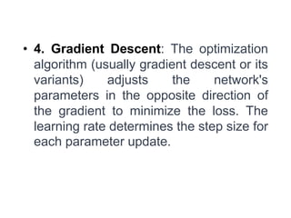
The document provides an overview of deep learning, covering fundamental concepts such as feedforward neural networks, gradient descent, and backpropagation. It discusses various types of neural networks including convolutional and recurrent networks, as well as advanced architectures like autoencoders and GANs. Key challenges such as unit saturation and the vanishing gradient problem are also addressed, with strategies for mitigation highlighted throughout.

1. UNIT- I
• Introduction
• Feed forward Neural networks
• Gradient descent and the back propagation algorithm
• Unit saturation
• the vanishing gradient problem
• and ways to mitigate it.
• RelU Heuristics for avoiding bad local minima Heuristics
for faster training
• Nestors accelerated gradient descent Regularization
• Dropout

2. Introduction to Deep Learning
• Deep learning is a subfield of artificial
intelligence (AI) and machine learning that
focuses on training artificial neural networks to
perform tasks that typically require human
intelligence.
• It has gained widespread attention and made
significant advancements in various
applications, including image recognition, natural
language processing, speech recognition, and
more.

3. Here are some common types of deep
learning:
Feedforward Neural
Networks (FNNs):
• These are the fundamental
building blocks of deep
learning. FNNs consist of an
input layer, one or more hidden
layers, and an output layer.
• Each layer contains nodes
(neurons) that process and
transform the data.
• FNNs are used for various
tasks, including regression and
classification.
Convolutional Neural
Networks (CNNs):
• CNNs are designed for
processing grid-like data, such
as images and videos.
• They use convolutional layers
to automatically learn features
from local regions of the input,
making them highly effective in
tasks like image classification,
object detection, and image
segmentation.

4. Common types of deep learning
(contd..)
Recurrent Neural
Networks (RNNs):
• RNNs are designed for
sequential data, such as time
series, text, and speech. They
have feedback connections,
allowing them to maintain a
memory of previous inputs.
• RNNs are suitable for tasks
like natural language
processing (NLP), machine
translation, and speech
recognition.
Long Short-Term Memory
(LSTM)
• LSTMs are a type of RNN
architecture designed to
capture long-range
dependencies in sequential
data more effectively.
• They use specialized memory
cells to store and update
information over longer
sequences, making them
suitable for tasks requiring
understanding of context over
time.

5. Common types of deep learning
(contd..)
Gated Recurrent Unit
(GRU):
• GRUs are another variant of
RNNs that address the
vanishing gradient problem,
like LSTMs.
• They are computationally more
efficient and often used for
similar sequence-based tasks
in NLP and speech
recognition.
Autoencoders:
• Autoencoders are neural
networks used for
unsupervised learning and
dimensionality reduction.
• They consist of an encoder
that maps input data to a
lower-dimensional
representation (encoding) and
a decoder that reconstructs the
original data from this
encoding.
• Autoencoders are used in
applications like image
denoising and anomaly
detection.

6. Common types of deep learning
(contd..)
Generative Adversarial
Networks (GANs):
• GANs consist of two neural
networks, a generator and a
discriminator, that compete
against each other.
• The generator tries to create
data that is indistinguishable
from real data, while the
discriminator tries to tell real
from fake.
• GANs are used for tasks like
image generation, style
transfer, and data
augmentation.
Transformer Models:
• Transformers have
revolutionized natural
language processing (NLP)
and have been adapted to
various other domains.
• They use a self-attention
mechanism to process input
data in parallel, making them
highly scalable and effective
for sequence-to-sequence
tasks.
• Notable transformer-based
models include BERT, GPT
(Generative Pre-trained
Transformer), and T5.

7. Common types of deep learning
(contd..)
Siamese Networks:
• These networks are designed
for tasks involving similarity or
distance measurement
between pairs of inputs.
• Siamese networks have two
identical subnetworks that
process each input and
produce embeddings that can
be compared to measure
similarity or dissimilarity.
Capsule Networks
(CapsNets):
• CapsNets are designed to
improve the shortcomings of
traditional CNNs, especially in
handling pose variations and
hierarchical features in images.
• They use capsules instead of
neurons to represent different
parts of an object.

8. Feed forward Neural networks
• Deep feedforward networks, also called feedforward neural
networks, or multilayer perceptrons (MLPs), are the
quintessential deep learning models.
• The goal of a feedforward network is to approximate some
function f∗.
• For example, for a classifier, y=f∗(x) maps an input x to a
category y.
• A feedforward network defines a mapping y=f(x;θ) and learns the
value of the parameters θ that result in the best function
approximation.
These models are called feedforward because information flows through
the function being evaluated from x, through the intermediate computations
used to define f, and finally to the output y. There are no feedback
connections in which outputs of the model are fed back into itself. When
feedforward neural networks are extended to include feedback
connections, they are called recurrent neural networks

9. Feed forward Neural networks (Contd.)
• Feedforward neural networks are often referred to as "networks"
because they are constructed by combining multiple functions.
• These networks are represented by a directed acyclic graph that
illustrates how these functions are interconnected.
• Typically, they are organized in a sequential manner, with functions
like f(1), f(2), and f(3) linked together in a chain, forming an overall
function f(x) = f(3)(f(2)(f(1)(x))).
• These chain-like structures are the most common configuration for
neural networks. In this context, each function, such as f(1), f(2), etc.,
is termed a layer of the network, with f(1) being the first layer, f(2) the
second layer, and so forth. They form the hidden layers.
• The overall length of the chain gives the depth of the model. The name
“deep learning” arose from this terminology. The final layer of a
feedforward network is called the output layer.
• Feedforward networks use the activation functions to compute the hidden
layer values.

11. Example: Learning XOR
• An example of a fully functioning feedforward network on a
very simple task: learning the XOR function.
• The XOR function (“exclusive or”) is an operation on two
binary values, x1andx2.
• When exactly one of these binary values is equal to 1, the
XOR function returns 1. Otherwise, it returns 0.
• The XOR function provides the target function y=f∗(x) that we
want to learn. Our model provides a function y=f(x;θ), and
our learning algorithm will adapt the parameters θ to make f
as similar as possible to f∗

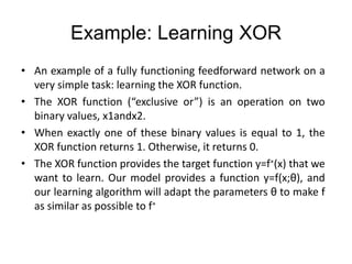
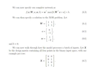
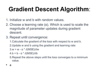
12. We want our network to perform correctly on the four points X = {[0,
0], [0,1],[1,0], and [1,1]}.
We will train the network on all four of these points.
The only challenge is to fit the training set.
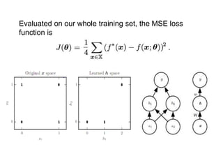
Evaluated on our whole training set, the MSE loss function is a
linear model, with θ consisting of w and b.
Our model is defined to be
f (x; w, b) = x T w + b.

14. Evaluated on our whole training set, the MSE loss
function is

17. To finish computing the value of h for each example, we apply the rectified
linear transformation: In this space, all the examples lie along a line with slope
1. As we move along this line, the output needs to begin at 0, then rise to 1,
then drop back down to 0. A linear model cannot implement such a function.

18. GRADIENT DESCENT & BACK
PROPAGATION
• Gradient descent and the backpropagation algorithm are
fundamental techniques used in training artificial neural
networks for various machine learning tasks, including
image recognition, natural language processing, and
more.
• Gradient Descent:
• Gradient descent is an optimization algorithm used to
minimize a loss function by adjusting the parameters
(weights and biases) of a machine learning model
iteratively. The idea is to find the set of parameters that
minimizes the error between the model's predictions and
the actual target values.

19. Here's a simple example of gradient
descent with a linear regression model:
• Objective: Minimize the mean squared error (MSE) loss for a
linear regression model.
• Linear Regression Model: The model has a single
parameter, a weight (w), and a bias (b). It predicts an output
(y_pred) given an input (x) as follows:
• y_pred = w * x + b
• Loss Function: The MSE loss for linear regression is defined
as:
• MSE = (1/n) * Σ(y_i - y_pred_i)^2
• Where:
• n is the number of data points.
• y_i is the actual target for the i-th data point.
• y_pred_i is the predicted output for the i-th data point.

20. Gradient Descent Algorithm:
1. Initialize w and b with random values.
2. Choose a learning rate (α). Which is used to scale the
magnitude of parameter updates during gradient
descent.
3. Repeat until convergence:
1.Calculate the gradient of the loss with respect to w and b.
2.Update w and b using the gradient and learning rate:
3.w = w - α * ∂(MSE)/∂w
4.b = b - α * ∂(MSE)/∂b
5.Repeat the above steps until the loss converges to a minimum
value.
• a

21. A simple example of gradient
descent using a one-dimensional
function.
• Suppose we want to minimize the
following quadratic function:
• f(x) = x^2
• The goal is to find the minimum value of
this function using gradient descent.

22. GD
• The gradient is:
• ∂f/∂x = 2x
• Update x using the gradient and the learning
rate:
• x = x - α * ∂f/∂x
1.Repeat steps 2 and 3 for a specified
number of iterations or until convergence.
• Let's perform a few iterations of gradient
descent:

24. As you can see, with each iteration, x
gets closer to 0, which is the minimum
of the function.
This process continues until the
convergence criteria are met or a
specified number of iterations are
reached.
In practice, gradient descent is used
to optimize more complex functions
with high-dimensional parameter
spaces, such as training neural
networks in deep learning.

25. Back Propagation Algorithm
• Backpropagation is a fundamental
algorithm used for training artificial neural
networks, particularly feedforward neural
networks with multiple layers (also known
as deep neural networks).
• It enables the network to learn from data
by iteratively adjusting its parameters
(weights and biases) to minimize a
predefined loss or error function.

26. Key Concepts in
Backpropagation:
1. Feedforward Pass: In the feedforward pass, input data is
propagated through the network layer by layer, resulting in an
output prediction. Each neuron in a layer calculates a weighted
sum of its inputs, applies an activation function, and passes the
result to the next layer.
2. Loss Function: A loss function (also known as a cost function)
quantifies the error between the network's predictions and the
actual target values. Common loss functions include mean
squared error (MSE) for regression tasks and cross-entropy for
classification tasks.
3. Backpropagation of Error: After the feedforward pass, the
network computes the gradient of the loss with respect to its
parameters (weights and biases) using the chain rule from calculus.
This gradient information is then used to update the parameters
during the optimization process.

27. • 4. Gradient Descent: The optimization
algorithm (usually gradient descent or its
variants) adjusts the network's
parameters in the opposite direction of
the gradient to minimize the loss. The
learning rate determines the step size for
each parameter update.

29. Example of Backpropagation:
• Let's consider training a feedforward neural
network for binary classification. The network
has one hidden layer with two neurons and
an output layer with a single neuron. We'll
use a simple dataset of two-dimensional
points (x1, x2) and binary labels (0 or 1) for
the example. The network's architecture is as
follows:
• Input layer: 2 neurons (corresponding to x1
and x2)
• Hidden layer: 2 neurons (with sigmoid
activation)
• Output layer: 1 neuron (with sigmoid

30. Steps in Backpropagation:
• Forward Pass:
• Input (x1, x2) is fed into the network.
• Calculate the weighted sum and apply the
sigmoid activation in the hidden layer.
• Calculate the weighted sum and apply the
sigmoid activation in the output layer.

31. 1. Loss Calculation:
1.Compute the loss (e.g., cross-entropy) between the predicted
output and the actual target label.
2. Backpropagation:
1.Calculate the gradient of the loss with respect to the output
layer's weighted sum and biases.
2.Backpropagate this gradient to the hidden layer and compute
gradients for its parameters.
3.Use these gradients to update the weights and biases in both
layers using gradient descent.
• Repeat:
• Repeat the above steps for a batch of training
examples (mini-batch) and iterate through the entire
dataset for multiple epochs.

33. Here's a simplified example of a
single training iteration:
• Forward Pass:
• Input (x1, x2) = (1.0, 0.5)
• Hidden layer:
• Weighted sum: z1 = w1 * x1 + w2 * x2 + b1
• Activation: a1 = sigmoid(z1)
• Similar calculations for neuron 2 in the hidden layer.
• Output layer:
• Weighted sum: z2 = w3 * a1 + w4 * a2 + b2
• Activation: a2 = sigmoid(z2)
• Loss Calculation:
• Calculate the cross-entropy loss between the
predicted output a2 and the actual label (0 or 1).

34. • Backpropagation:
• Compute gradients for output layer parameters (e.g.,
w3, w4, b2).
• Propagate gradients backward to the hidden layer,
compute gradients for its parameters (e.g., w1, w2,
b1).
• Update all weights and biases using gradient
descent.
• This process is repeated for multiple training
iterations until the network's parameters
converge, and the loss reaches a satisfactory
minimum.

35. UNIT SATURATION
• Unit saturation, also known as saturation of a neural unit, is a
phenomenon that occurs when the activation function of a neuron
reaches extreme values, typically 0 or 1, and remains there for
most input values.
• In other words, the neuron saturates when its input is either very
large (positive or negative) or very close to zero, causing the
output of the neuron to become insensitive to further changes in
input.
• This can pose problems during training because the gradients
with respect to the weights may become very small, leading to
slow convergence or vanishing gradients.
• Unit saturation is often associated with activation functions like
sigmoid and hyperbolic tangent(tanh)

36. • Sigmoid Activation Function: The sigmoid function
is defined as follows:
• σ(x) = 1 / (1 + exp(-x))
• When x is very large (positive or negative), σ(x) approaches
1 or 0, respectively.
• When x is close to 0, σ(x) is approximately 0.5.
• Example of Unit Saturation:
• Consider a neural network with a sigmoid activation
function and a weight (w) connected to a neuron. Let's say
that during training, the network encounters an input value
(x) of 10 for this neuron:
• x = 10

37. • Now, let's compute the output of the neuron using the sigmoid function:
• σ(10) ≈ 0.9999546
• At this point, the neuron has effectively saturated. Even small changes in w or x
may not significantly affect the neuron's output because the output is already
close to 1.
• As a result:
• The gradient with respect to w (needed for weight updates during training)
becomes very small, causing slow learning or convergence issues.
• The neuron is not effectively contributing to the learning process since it
responds similarly to large variations in input.
• In practice, this phenomenon can lead to challenges in training deep neural
networks, especially when using activation functions like sigmoid or tanh. To
mitigate unit saturation, other activation functions such as ReLU (Rectified
Linear Unit) or variants like Leaky ReLU and Parametric ReLU are often used.
• These activation functions do not saturate as quickly for positive inputs and
allow gradients to flow more effectively during training, which can lead to
faster convergence and better learning.