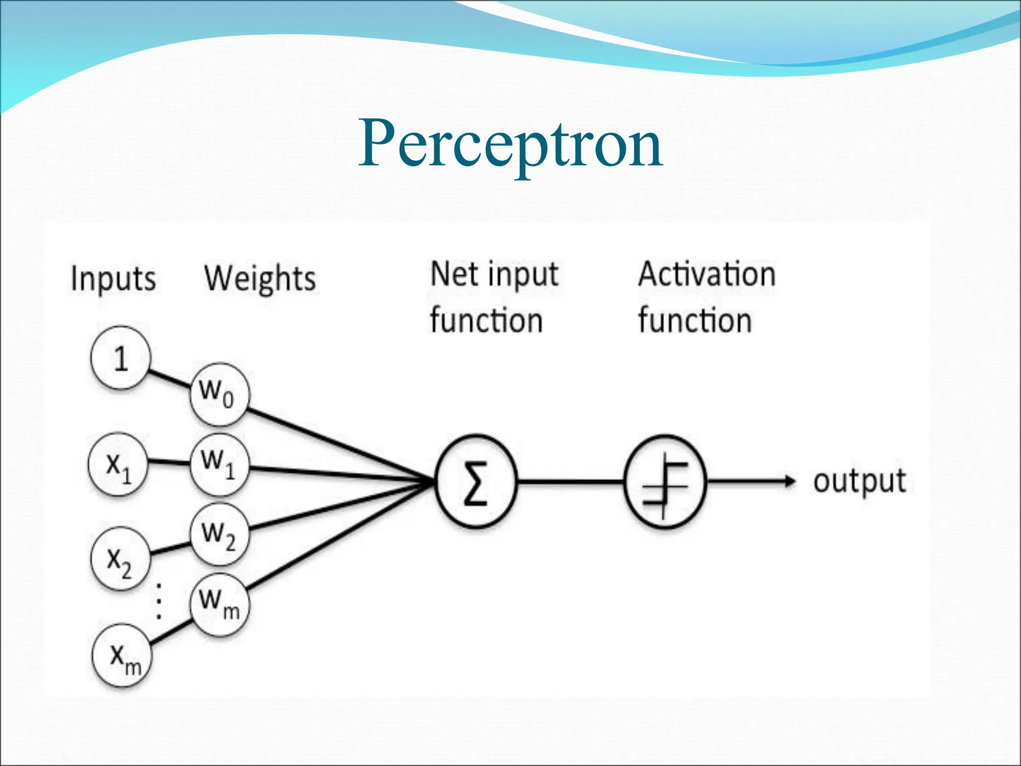
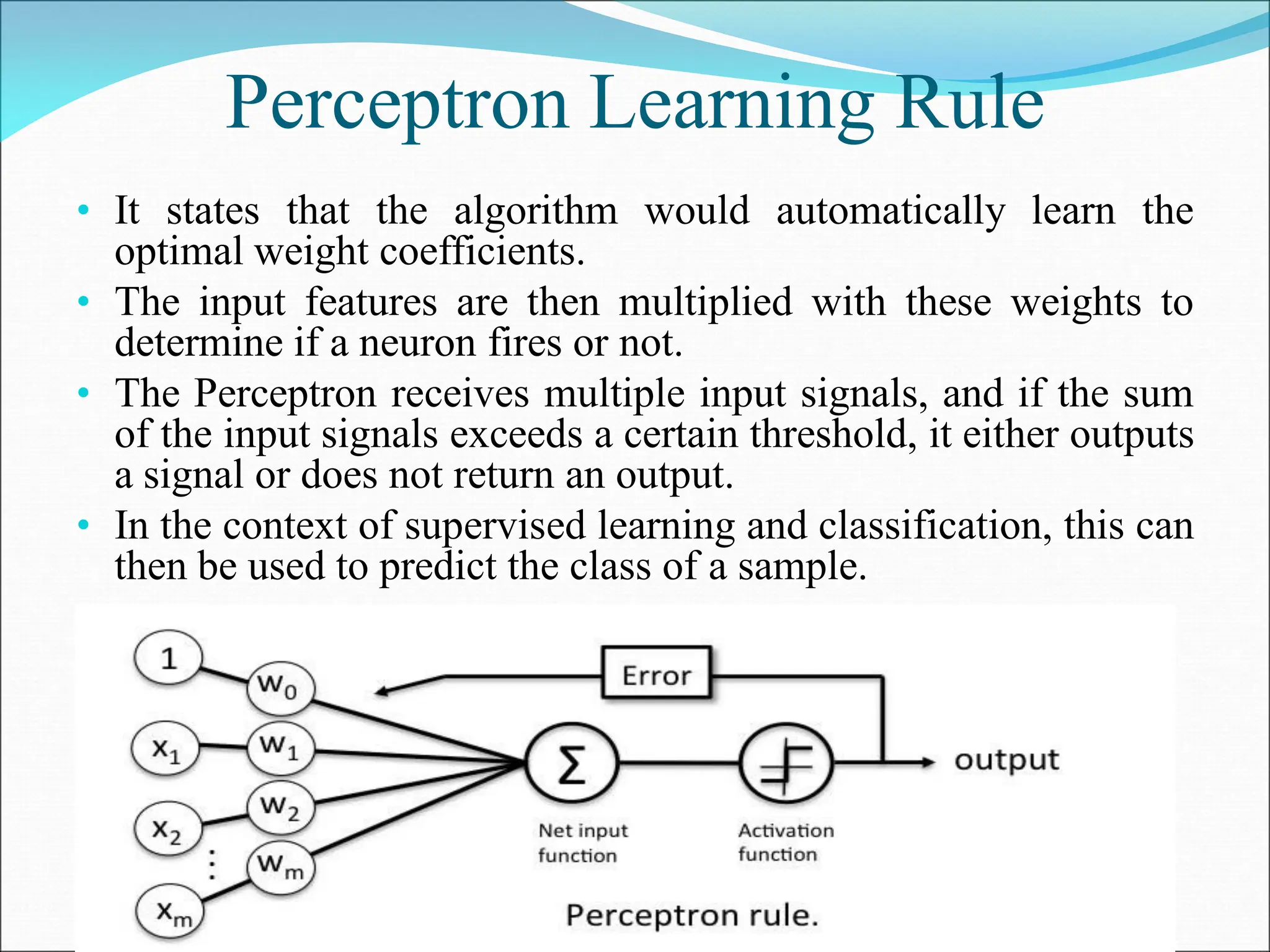
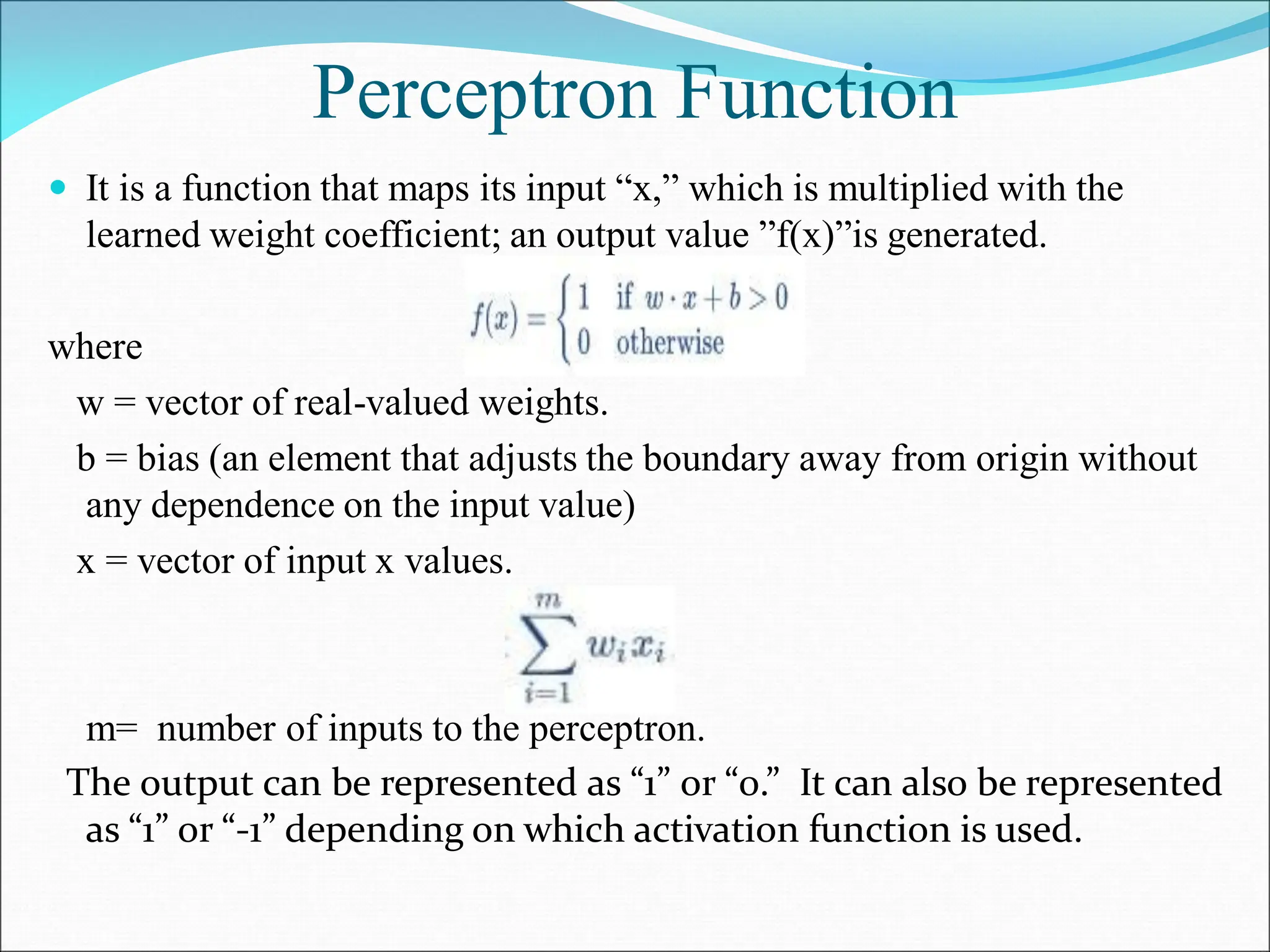
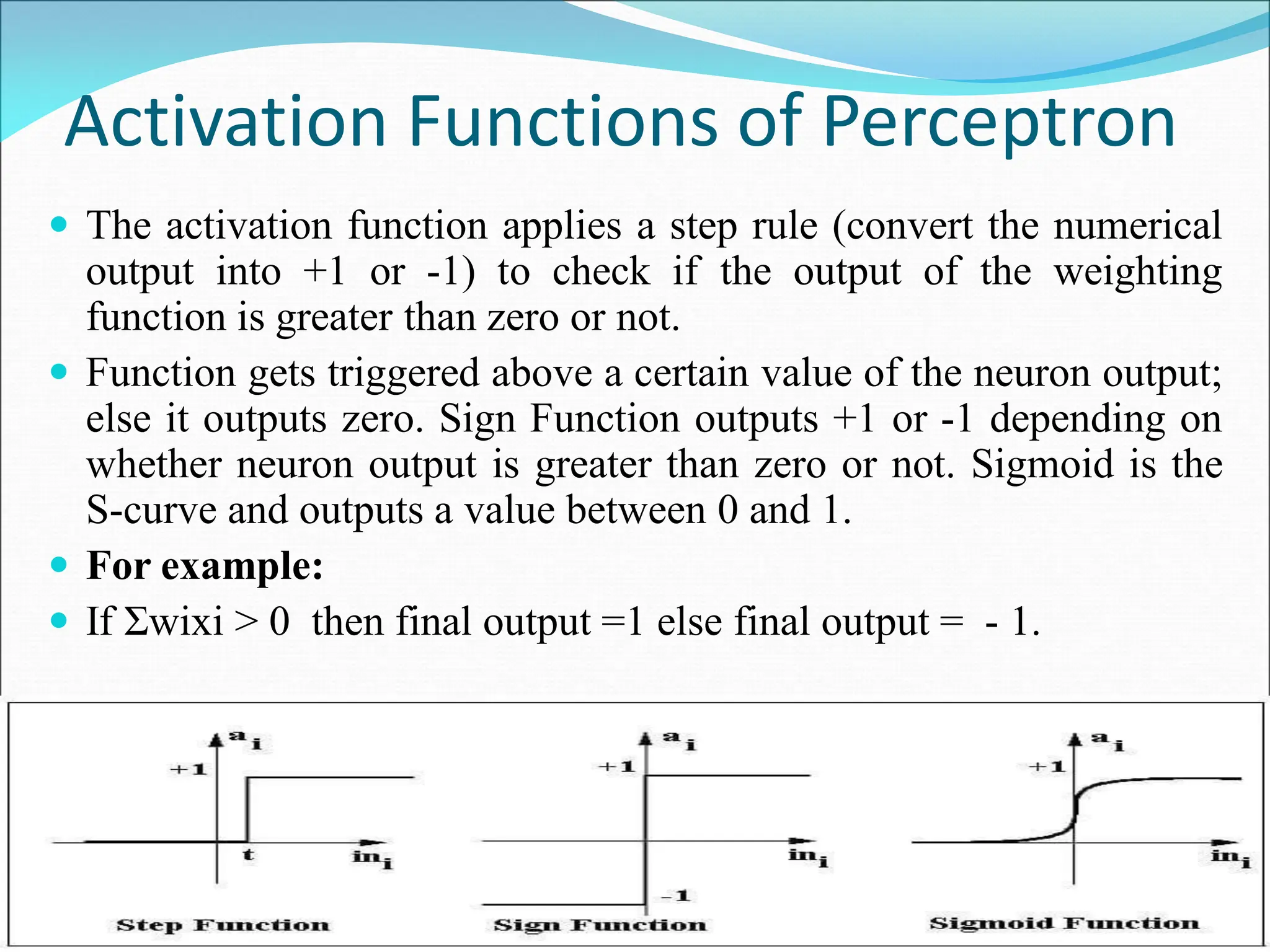
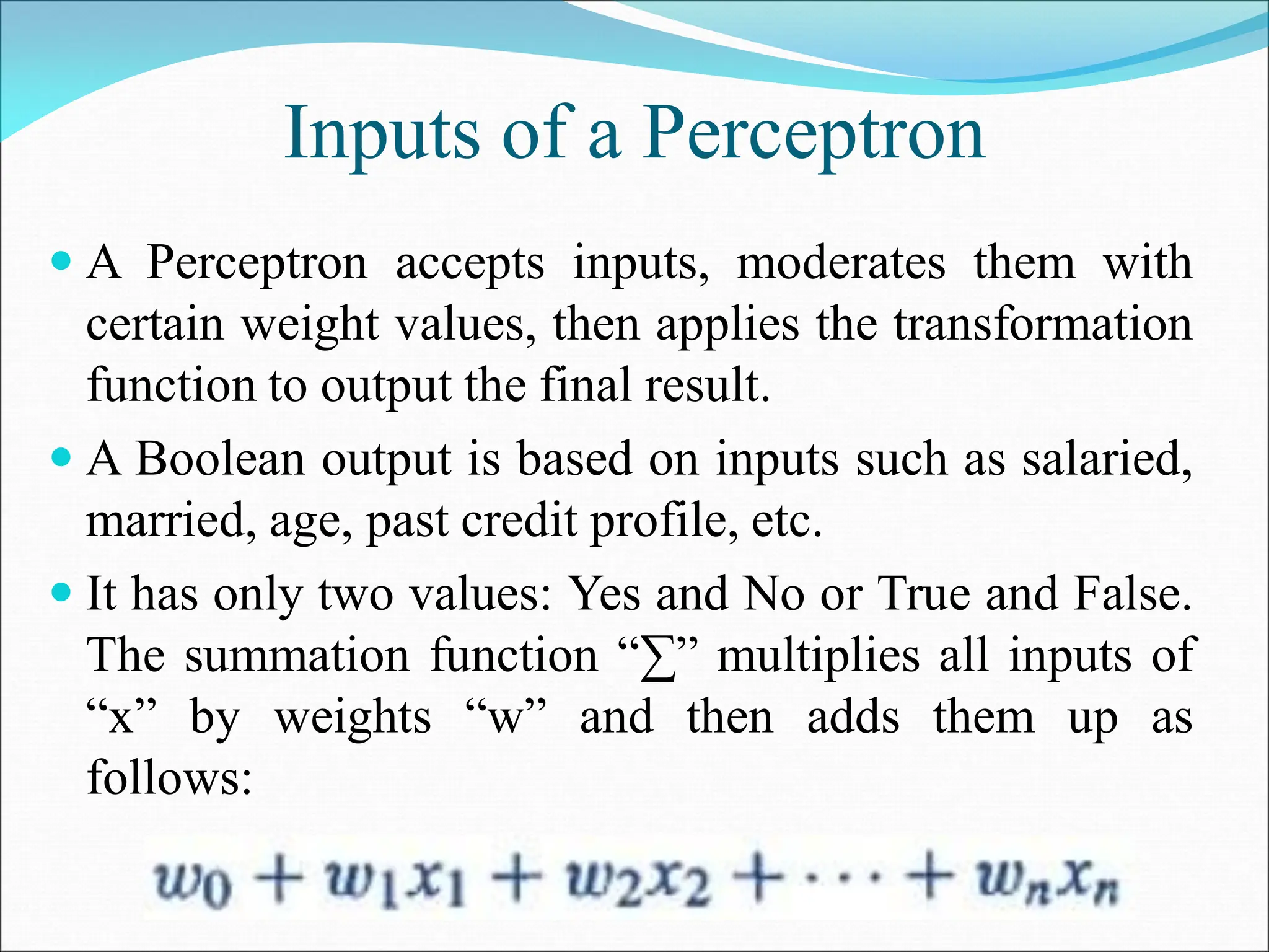
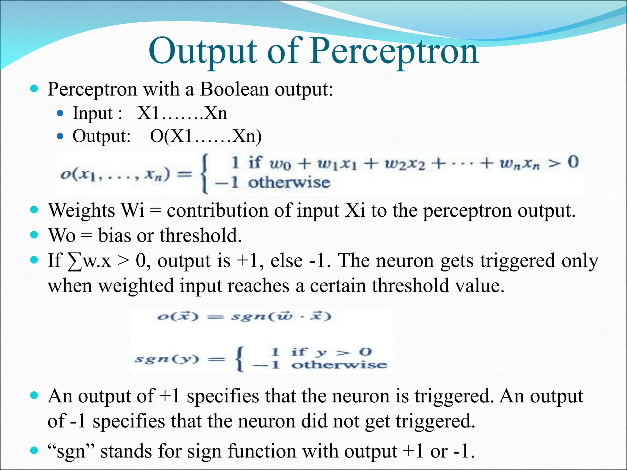
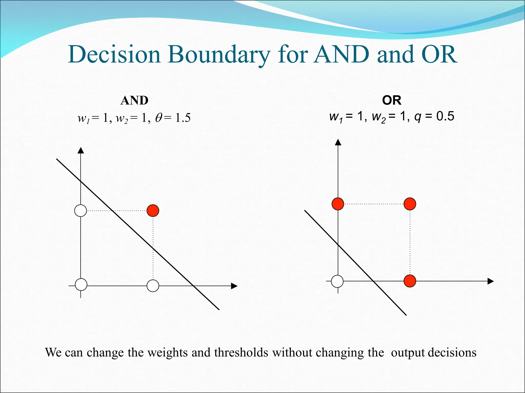
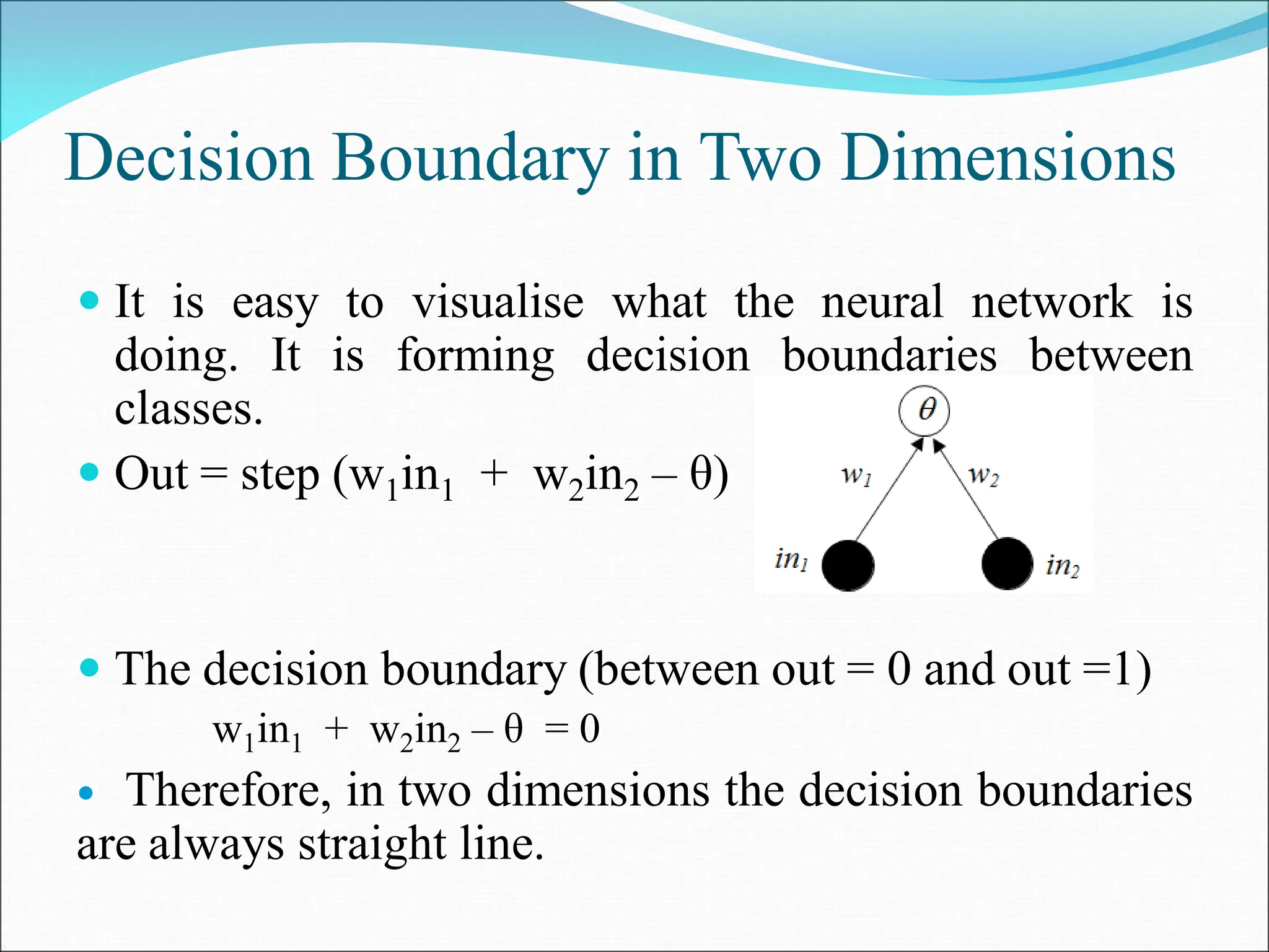
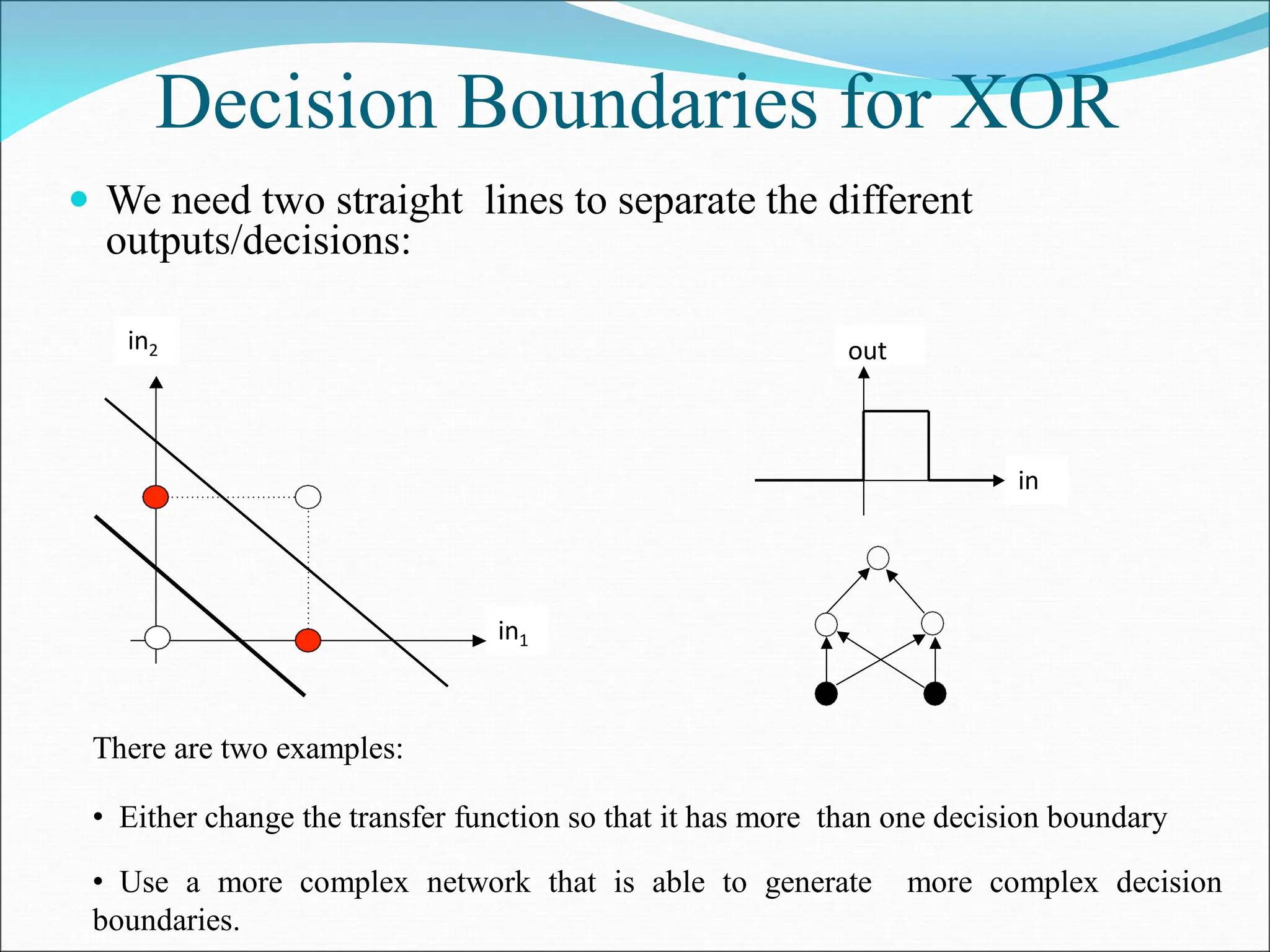
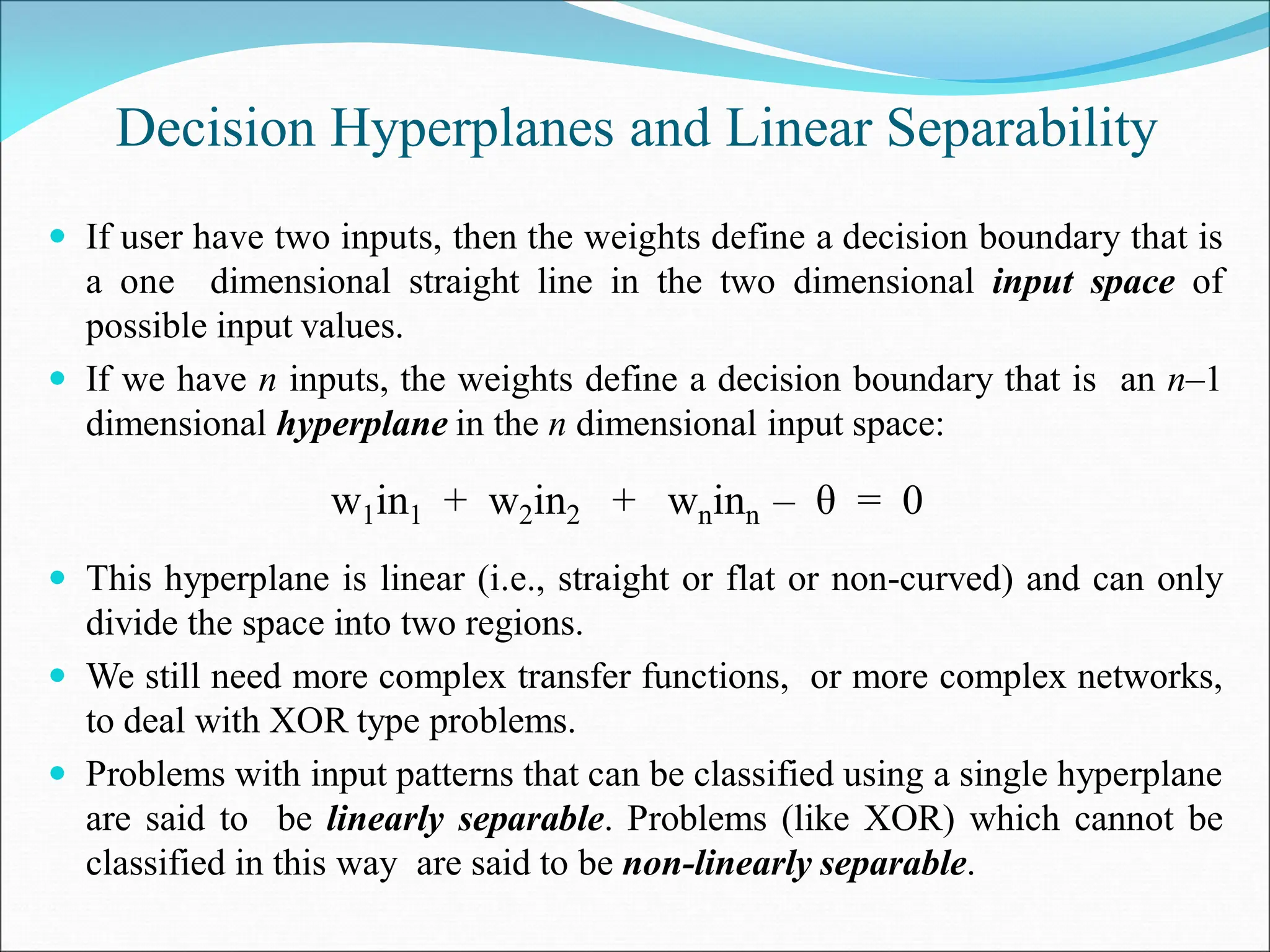
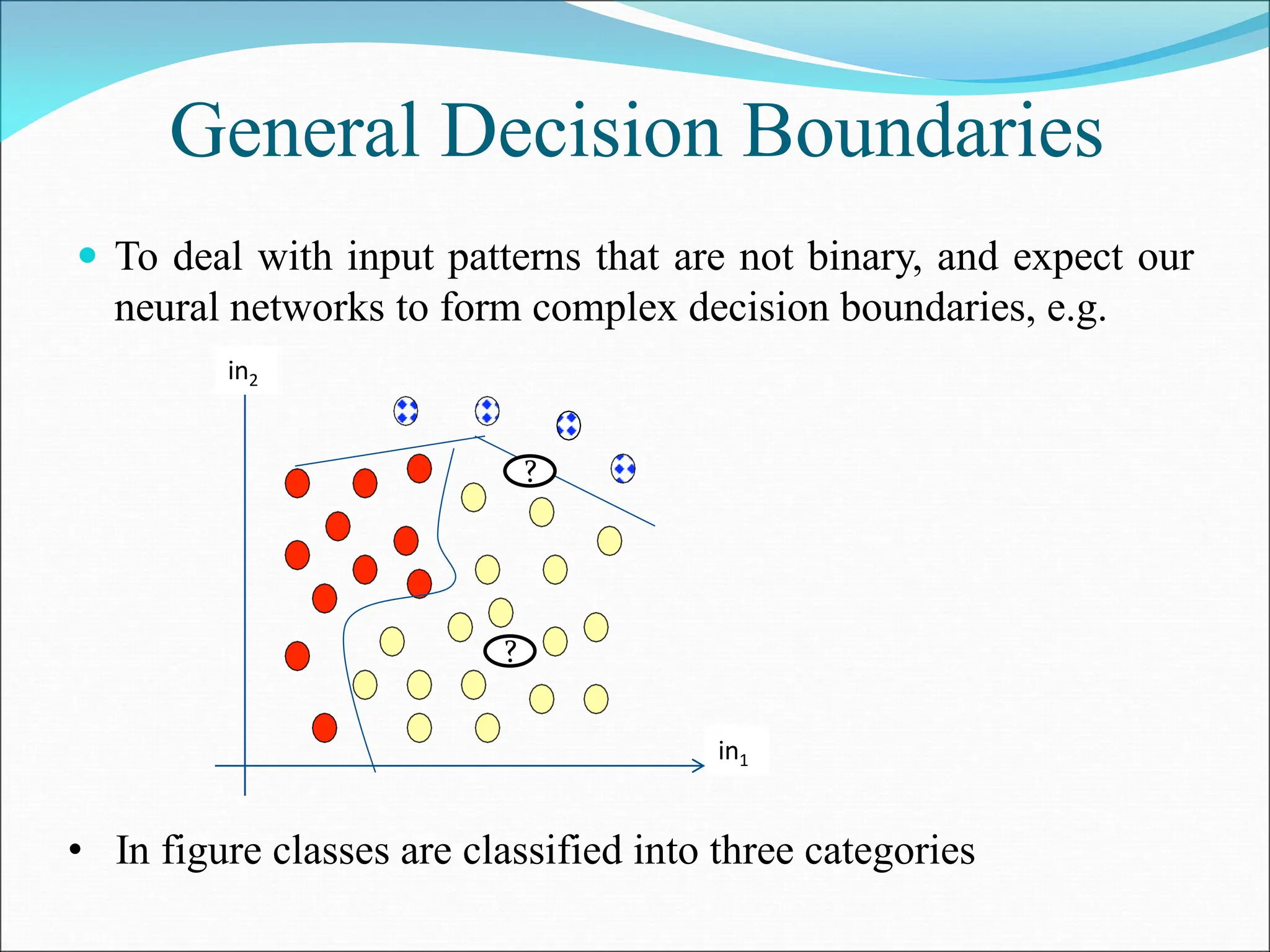
- A perceptron is a simple model of an artificial neuron that can be used for classification problems. It takes weighted inputs, sums them, and outputs 1 if the sum exceeds a threshold or 0 otherwise. - Perceptrons can only learn linearly separable patterns. Multilayer perceptrons with more than one layer have greater processing power to learn nonlinear patterns. - The perceptron learning rule adjusts the weights to correctly classify training examples by shifting the decision boundary in small steps. This allows the network to learn the optimal weights from data.

1. Dr. P. K. Chaurasia
Associate Professor,
Department of Computer Science and
Information Technology
MGCUB, Motihari, Bihar

2. Introduction
• A perceptron is a simple model of a biological neuron in an
artificial neural network.
• The perceptron algorithm was designed to classify visual
inputs, categorizing subjects into one of two types and
separating groups with a line.
• Classification is an important part of machine learning and
image processing.
• Perceptron was introduced by Frank Rosenblatt in 1957.

3. cont…
• Each perceptron sends multiple signals, one signal going to
each perceptron in the next layer. For each signal,
the perceptron uses different weights.
• One difference between an MLP and a neural network is
that in the classic perceptron, the decision function is a
step function and the output is binary.
• Perceptron is a single layer neural network and a multi-
layer perceptron is called Neural Networks.
• Perceptron is a linear classifier (binary).
• It is used in supervised learning. It helps to classify the
given input data.

4. Biological Neurons
Cell nucleus or soma processes the information received from
dendrites.
Axon is a cable that is used by neurons to send information.
Synapse is the connection between an axon and other neuron
dendrites.

5. Rise of Artificial Neurons
• Researchers Warren McCullock and Walter Pitts published their
first concept of simplified brain cell in 1943.
• This was called McCullock-Pitts (MCP) neuron.
• They described such a nerve cell as a simple logic gate with
binary outputs.
• Multiple signals arrive at the dendrites and are then integrated into
the cell body.
• If the accumulated signal exceeds a certain threshold, an output
signal is generated that will be passed on by the axon.

6. Artificial Neurons
 An artificial neuron is a mathematical function based on a model
of biological neurons, where each neuron takes inputs, weighs
them separately, sums them up and passes this sum through a
nonlinear function to produce output.

7. Artificial Neurons
• It has the following characteristics:
 A neuron is a mathematical function modeled on the
working of biological neurons.
 It is an elementary unit in an artificial neural network.
 One or more inputs are separately weighted.
 Inputs are summed and passed through a nonlinear function
to produce output.
 Every neuron holds an internal state called activation signal.
 Each connection link carries information about the input
signal.
 Every neuron is connected to another neuron via connection
link.

8. Biological Neurons vs. Artificial Neurons
 The biological neuron is analogous to artificial
neurons in the following terms:
Biological Neurons Artificial Neurons
Cell Nucleus (Soma) Node
Dendrites Input
Synapse Weights or interconnections
Axon Output

9. Training Neural Network
 The neural network is a simple Perceptron, or a much more
complicated multi-layer network with special activation functions.
 We need to develop a systematic procedure for determining
appropriate connection weights.
 The network learn the appropriate weights from a representative
set of training data.
 The simplest cases, however, direct computation of the weights
are unmanageable.
 A good process is to start off with random initial weights and
adjust them in small steps until the required outputs are
generated.

10. Perceptron
• A perceptron is a neural network unit that does certain
computations to detect features or business
intelligence in the input data.
• A Perceptron is an algorithm for supervised learning
of binary classifiers.
• This algorithm enables neurons to learn and processes
elements in the training set one at a time.
• A single artificial neuron that computes its weighted
input and uses a threshold activation function.

11. Perceptron

12. Types of Perceptron
• There are two types of perceptrons:
• Single layer
• Multilayer.
• Single layer Perceptrons can learn only linearly separable
patterns.
• Multilayer Perceptrons or feedforward neural networks with
two or more layers have the greater processing power.
• The Perceptron algorithm learns the weights for the input
signals in order to draw a linear decision boundary.
• This enables you to distinguish between the two linearly
separable classes +1 and -1.

13. Perceptron Learning
 The decision boundaries are hyperplanes, learning as the process of
shifting around the hyperplanes, until each training pattern is
classified correctly.
 Somehow, we need to formalise that process of “shifting around” into
a systematic algorithm that can easily be implemented on a computer.
 The “shifting around” can be split up into a number of small steps.
 If the network weights at time t are wij(t) , then the shifting process
corresponds to moving them by a small amount wij(t) so that at time
t+1 we have weights.
wij (t +1) = wij (t ) + wij (t)
 It is convenient to treat the thresholds as weights, as discussed
previously, so we don’t need separate equations for them..

14. Perceptron Learning Rule
• It states that the algorithm would automatically learn the
optimal weight coefficients.
• The input features are then multiplied with these weights to
determine if a neuron fires or not.
• The Perceptron receives multiple input signals, and if the sum
of the input signals exceeds a certain threshold, it either outputs
a signal or does not return an output.
• In the context of supervised learning and classification, this can
then be used to predict the class of a sample.

15. Perceptron Function
 It is a function that maps its input “x,” which is multiplied with the
learned weight coefficient; an output value ”f(x)”is generated.
where
w = vector of real-valued weights.
b = bias (an element that adjusts the boundary away from origin without
any dependence on the input value)
x = vector of input x values.
m= number of inputs to the perceptron.
The output can be represented as “1” or “0.” It can also be represented
as “1” or “-1” depending on which activation function is used.

16. Activation Functions of Perceptron
 The activation function applies a step rule (convert the numerical
output into +1 or -1) to check if the output of the weighting
function is greater than zero or not.
 Function gets triggered above a certain value of the neuron output;
else it outputs zero. Sign Function outputs +1 or -1 depending on
whether neuron output is greater than zero or not. Sigmoid is the
S-curve and outputs a value between 0 and 1.
 For example:
 If Σwixi > 0 then final output =1 else final output = - 1.

17. Inputs of a Perceptron
 A Perceptron accepts inputs, moderates them with
certain weight values, then applies the transformation
function to output the final result.
 A Boolean output is based on inputs such as salaried,
married, age, past credit profile, etc.
 It has only two values: Yes and No or True and False.
The summation function “∑” multiplies all inputs of
“x” by weights “w” and then adds them up as
follows:

18. Output of Perceptron
 Perceptron with a Boolean output:
 Input : X1…….Xn
 Output: O(X1……Xn)
 Weights Wi = contribution of input Xi to the perceptron output.
 Wo = bias or threshold.
 If ∑w.x > 0, output is +1, else -1. The neuron gets triggered only
when weighted input reaches a certain threshold value.
 An output of +1 specifies that the neuron is triggered. An output
of -1 specifies that the neuron did not get triggered.
 “sgn” stands for sign function with output +1 or -1.

19. Decision Boundary
 The weight vector is relevant to the decision
boundary.
 The weight vector points in the direction of the vector
which should produce an output of 1.
 Vector with the positive output are on the right side of the
decision boundary.
 If w pointed in the opposite direction, the dot products of all input
vectors would have the opposite sign.
 Would result in same classification but opposite labels.
 The bias determines the position of the boundary.
 WTP + b = 0 using one point on the decision boundary
to find b.

20. Decision Boundary in Two Dimensions
 It is easy to visualise what the neural network is
doing. It is forming decision boundaries between
classes.
 Out = step (w1in1 + w2in2 – θ)
 The decision boundary (between out = 0 and out =1)
w1in1 + w2in2 – θ = 0
 Therefore, in two dimensions the decision boundaries
are always straight line.

21. Decision Boundary for AND and OR
We can change the weights and thresholds without changing the output decisions
OR
w1 = 1, w2 = 1, q = 0.5
AND
w1 = 1, w2 = 1,  = 1.5

22. Decision Boundaries for XOR
 We need two straight lines to separate the different
outputs/decisions:
in1
in2
in
out
There are two examples:
• Either change the transfer function so that it has more than one decision boundary
• Use a more complex network that is able to generate more complex decision
boundaries.

23. Decision Hyperplanes and Linear Separability
 If user have two inputs, then the weights define a decision boundary that is
a one dimensional straight line in the two dimensional input space of
possible input values.
 If we have n inputs, the weights define a decision boundary that is an n–1
dimensional hyperplane in the n dimensional input space:
 This hyperplane is linear (i.e., straight or flat or non-curved) and can only
divide the space into two regions.
 We still need more complex transfer functions, or more complex networks,
to deal with XOR type problems.
 Problems with input patterns that can be classified using a single hyperplane
are said to be linearly separable. Problems (like XOR) which cannot be
classified in this way are said to be non-linearly separable.
w1in1 + w2in2 + wninn – θ = 0

24. General Decision Boundaries
 To deal with input patterns that are not binary, and expect our
neural networks to form complex decision boundaries, e.g.
in1
in2
?
?
• In figure classes are classified into three categories

25. Learning and Generalization
 A network produce outputs for input patterns that was not
originally set up to classify (shown with question marks), though
those classifications may be incorrect.
 There are two important aspects of the network’s operation :
 Learning: The network must learn decision boundaries from a set of
training patterns so that these training patterns are classified correctly.
 Generalization: After training, the network must also be able to
generalize, i.e. correctly classify test patterns it has never seen before.
 Sometimes, the training data may contain errors (e.g., noise in the
experimental determination of the input values, or incorrect
classifications). In this case, learning the training data perfectly
may make the generalization worse.

26. Generalization in Classification
 The objective of the neural network is to learn a
classification decision boundary:
in1
in2
in1
in2
The objective is to get the network to generalize to classify new inputs appropriately. If
the training data contains noise, we don’t necessarily want the training data to be
classified totally accurately, as that is likely to reduce the generalization ability.

27. Generalization in Function Approximation
 We wish to recover a function for which we only have
noisy data samples:
in1
in2
• The neural network output give better representation of the under-lying
function if its output curve does not pass through all the data points.
• A larger error on the training data is likely to lead to better generalization.

28. Review Questions
 What is the difference between biological neurons and
artificial neurons?
 What is perceptron? What are the different types of
perceptron?
 What is decision boundary? Explain.
 What are the two important aspects of network
operation?
 What is classification decision boundary?
 What is general decision boundary? Explain.

29. References
 List of Books
 Understanding Machine Learning: From Theory to Algorithms.
 Introductory Machine Learning notes
 Foundations of Machine Learning
 List of websites referred:
 https://www.simplilearn.com/what-is-perceptron-tutorial.
 https://www.cs.bham.ac.uk/~pxt/NC/l4_JB.pdf
 https://www.cs.cmu.edu/afs/cs.cmu.edu/academic/class/15381-
f01/www/handouts/110601.pdf
 https://www.simplilearn.com/what-is-perceptron-tutorial