ann ppt

1. Unit-2 Perceptron

2. Unit Explains
• Introduction
• Perceptron Architecture
• Perceptron learning rule
• Complexity of perceptron learning
• Computational limits of perceptron
• Linearly separable functions
• Learning XOR
• FFN
• Backpropogation

3. Introduction to Perceptron
• Perceptron is one of the simplest artificial neural
network architectures, introduced by Frank Rosenblatt in 1957. It is
primarily used for binary classification.
• proved to be highly effective in solving specific classification
problems, laying the groundwork for advancements in AI and machine
learning.

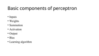
4. What is perceptron?
• Perceptron is a type of neural network that performs binary
classification that maps input features to an output decision, usually
classifying data into one of two categories, such as 0 or 1.
• consists of a single layer of input nodes that are fully connected to a
layer of output nodes.
• good at learning linearly separable patterns.
• utilizes a variation of artificial neurons called Threshold Logic Units
(TLU), which were first introduced by McCulloch and Walter Pitts in
the 1940s.
• This foundational model has played a crucial role in the development
of more advanced neural networks and machine learning algorithms.

5. Types of perceptron

6. Basic components of perceptron
• Inputs
• Weights
• Summation
• Activation
• Output
• Bias
• Learning algorithm

7. How it works?

9. How does it learns?
• The perceptron updates its weights during training to improve
accuracy.
Learning Rule:

11. Perceptron Architecture

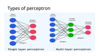
12. Single Neuron perceptron
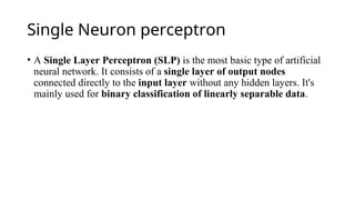
• A Single Layer Perceptron (SLP) is the most basic type of artificial
neural network. It consists of a single layer of output nodes
connected directly to the input layer without any hidden layers. It's
mainly used for binary classification of linearly separable data.

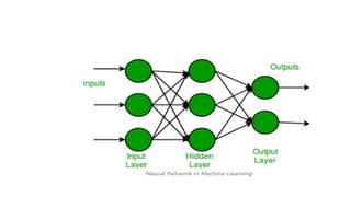
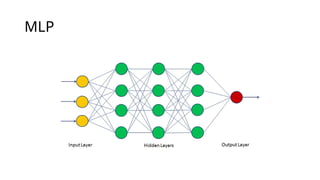
14. Multineuron perceptron
• A multi-layer perceptron (MLP) is a type of artificial neural network
consisting of multiple layers of neurons. The neurons in the MLP
typically use nonlinear activation functions, allowing the network to
learn complex patterns in data.

15. MLP

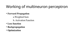
16. Working of multineuron perceptron
• Forward Propagation
a.Weighted Sum
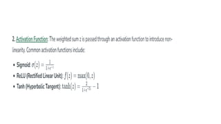
b. Activation Function
• Loss function
• Backpropogation
• Optimization

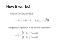
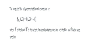
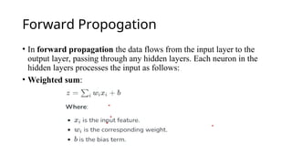
17. Forward Propogation
• In forward propagation the data flows from the input layer to the
output layer, passing through any hidden layers. Each neuron in the
hidden layers processes the input as follows:
• Weighted sum:

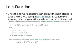
19. Loss Function
• Once the network generates an output the next step is to
calculate the loss using a loss function. In supervised
learning this compares the predicted output to the actual
label.

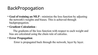
20. BackPropogation
• Goal of training an MLP - minimize the loss function by adjusting
the network's weights and biases. This is achieved through
backpropogation.
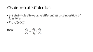
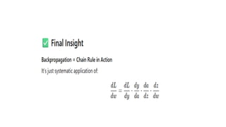
• Gradient Calculation :
The gradients of the loss function with respect to each weight and
bias are calculated using the chain rule of calculus.
• Error Propogation:
Error is propagated back through the network, layer by layer.

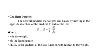
21. • Gradient Descent:
The network updates the weights and biases by moving in the
opposite direction of the gradient to reduce the loss
Where:
• w is the weight.
• ηis the learning rate.
• ∂L/∂w​is the gradient of the loss function with respect to the weight.

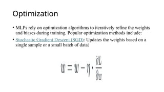
22. Optimization
• MLPs rely on optimization algorithms to iteratively refine the weights
and biases during training. Popular optimization methods include:
• Stochastic Gradient Descent (SGD): Updates the weights based on a
single sample or a small batch of data:

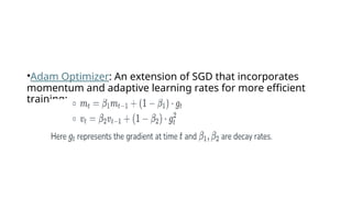
23. •Adam Optimizer: An extension of SGD that incorporates
momentum and adaptive learning rates for more efficient
training:

24. • Advantages of Multi Layer Perceptron
• Versatility: MLPs can be applied to a variety of problems, both classification
and regression.
• Non-linearity: Using activation functions MLPs can model complex, non-
linear relationships in data.
• Parallel Computation: With the help of GPUs, MLPs can be trained quickly
by taking advantage of parallel computing.
• Disadvantages of Multi Layer Perceptron
• Computationally Expensive: MLPs can be slow to train especially on large
datasets with many layers.
• Prone to Overfitting: Without proper regularization techniques they can
overfit the training data, leading to poor generalization.
• Sensitivity to Data Scaling: They require properly normalized or scaled data
for optimal performance.

25. Perceptron learning rule

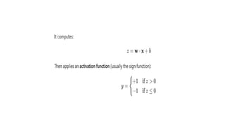
26. Constructing learning rule
• The perceptron is the simplest type of artificial neural network — a
single-layer model that makes decisions by weighing inputs.
• Basic model:
• Given:
• Input vector: x=[x1,x2,...,xn]
• Weight vector: w=[w1,w2,...,wn]
• Bias: b

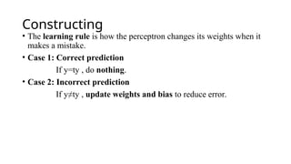
28. Constructing
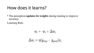
• The learning rule is how the perceptron changes its weights when it
makes a mistake.
• Case 1: Correct prediction
If y=ty , do nothing.
• Case 2: Incorrect prediction
If y≠ty , update weights and bias to reduce error.

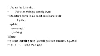
29. • Update the formula:
• For each training sample (x,t):
• Standard form (bias handled separately):
If y≠ty ,
• update:
w←w+ηtx
b←b+ηt
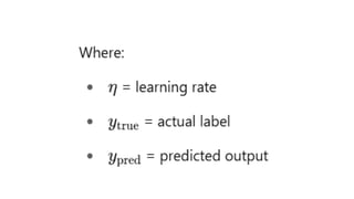
Where:
• η is the learning rate (a small positive constant, e.g., 0.1)
• t {+1,−1} is the
∈ true label

30. Unified learning rule

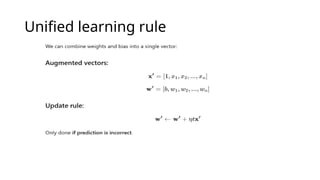
31. Benefits
• No need to handle bias separately.
• Simpler implementation.
• More elegant mathematical formulation.

32. Training multi neuron perceptron
• Training a multineuron perceptron means working with a single-
layer neural network that has multiple output neurons — each
neuron learning to detect a different pattern or class.
• This is referred to as SLFN.
• when using the Perceptron Learning Rule, each output neuron
behaves independently.

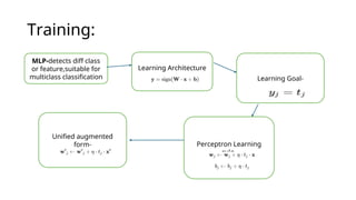
33. Training:
MLP-detects diff class
or feature,suitable for
multiclass classification
Learning Architecture
- Learning Goal-
Perceptron Learning
rule-
Unified augmented
form-

34. Complexity of perceptron learning

35. Computational limits of perceptron

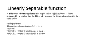
36. Linearly Separable function
A function is linearly separable if its output classes (typically 0 and 1) can be
separated by a straight line (in 2D) or a hyperplane (in higher dimensions) in the
input space.
In simpler terms:
There exists a linear function f(x)=w x+b
⋅
such that:
•f(x)>0f(x) > 0f(x)>0 for all inputs in class 1
•f(x)<0f(x) < 0f(x)<0 for all inputs in class 0

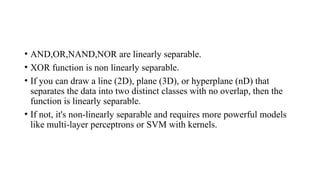
37. • AND,OR,NAND,NOR are linearly separable.
• XOR function is non linearly separable.
• If you can draw a line (2D), plane (3D), or hyperplane (nD) that
separates the data into two distinct classes with no overlap, then the
function is linearly separable.
• If not, it's non-linearly separable and requires more powerful models
like multi-layer perceptrons or SVM with kernels.

38. Learning XOR
• A single layer perceptron cannot learn XOR.
• So lets use Multilayer perceptron or Kernal method to learn
XOR ,since it is nonlinear.

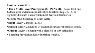
39. How to Learn XOR
• Use a Multi-Layer Perceptron (MLP):An MLP has at least one
hidden layer and nonlinear activation functions (e.g., ReLU or
sigmoid).This lets it create nonlinear decision boundaries.
•Simple MLP Structure to Learn XOR
•Input Layer: 2 inputs (x , x ),
₁ ₂
•Hidden Layer: 2 neurons with a nonlinear activation(likesigmoid)
•Output Layer: 1 neuron with a sigmoid or step activation
• Learning ProcessRandomly initialize weights.

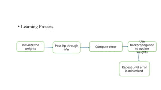
40. • Learning Process
Initialize the
weights
Pass i/p through
n/w
Compute error
Use
backpropogation
to update
weights
Repeat until error
is minimized

41. FeedForward Networks
• Information flows in one direction
• Without loops
• mainly used for pattern recognition tasks like image and speech
classification.
• For example :
in a credit scoring system, banks use an FNN which analyze
users financial profiles such as income, credit history and spending
habits to determine their creditworthiness.

42. Structure of feed forward neural n/w

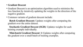
43. • Gradient Descent
• Gradient Descent is an optimization algorithm used to minimize the
loss function by iteratively updating the weights in the direction of the
negative gradient.
• Common variants of gradient descent include:
Batch Gradient Descent: Updates weights after computing the
gradient over the entire dataset.
Stochastic Gradient Descent (SGD): Updates weights for each
training example individually.
Mini-batch Gradient Descent: It Updates weights after computing
the gradient over a small batch of training examples.

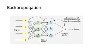
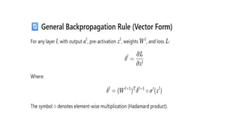
44. BackPropogation
• known as "Backward Propagation of Errors" is a method used to train
neural network .
• goal ---reduce the difference between the model’s predicted output
and the actual output by adjusting the weights and biases in the
network.
• works iteratively to adjust weights and bias to minimize the cost
function

45. Backpropogation

47. Chain of rule Calculus
• the chain rule allows us to differentiate a composition of
functions.
• If: = ( ( ))
𝑦 𝑓 𝑔 𝑥
then

48. Applying chain rule

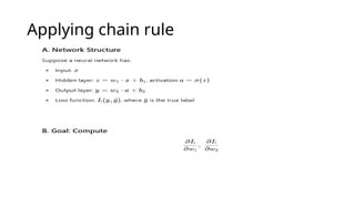
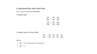
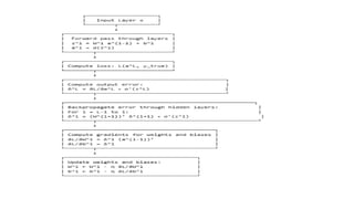
52. Bpcomputation in fully connected
multilayer Perceptron
• calculates how the loss changes with respect to the weights and biases
in each layer using the chain rule of calculus, and then updates them
using gradient descent.