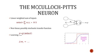
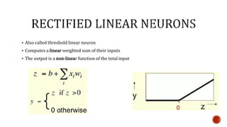
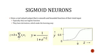
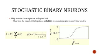
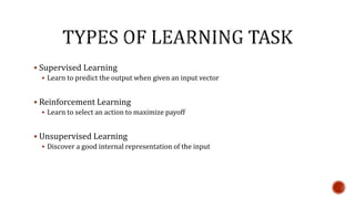
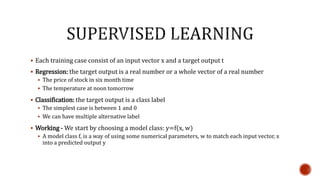
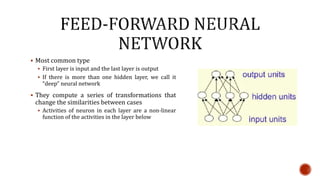
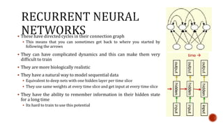
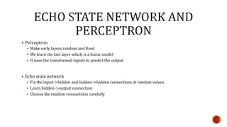
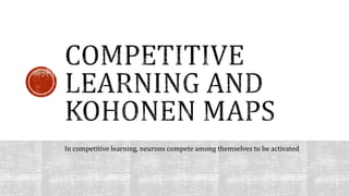
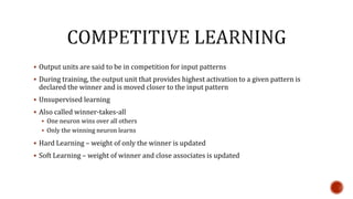
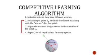
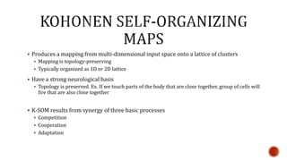
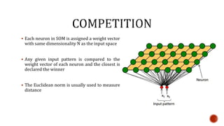
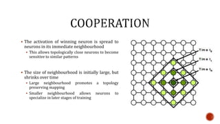
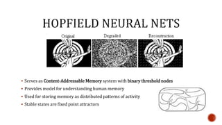
SlideShare a Scribd company logo
1 of 100
 Its very hard to write programs that solve problems like recognizing a 3D
object from a novel viewpoint.
 Even if we could have written such a program, it would have been very complicated
 Its hard to write a program that computes credit card fraudulent
 There are no specific rules that are simple and reliable. We need to combine a large
number of weak rules
 Fraud is a moving target. The program needs to keep changing
 Instead of writing programs for a specific task, we collect a lot of examples
that specify the correct output for a given input
 The machine learning algorithm then takes these examples and produces a
program that does the job
 Looks very different from a typical program
 Program works well for new cases and the ones that we train it on
 If the data changes, the program can change by training on the new data
 Massive amount of computation is now cheaper than paying for the code
 To study how the brain actually works
 It very big and complicated. So, we need the use of computer simulation
 To understand the style of parallel computation inspired by neurons and
their adaptive connection
 Very different from sequential connection
 Should be good at things that the brain is good at. Ex. Vision
 Should be bad at thing the brain is bad at. Ex. Computation 24 X 44
 To solve practical problems by using novel learning algorithms inspired by
brain
 Revolutionary Idea: think of neural tissue as circuits performing mathematical
computation
 Linear weighted sum of inputs
 Non-linear, possibly stochastic transfer function
 Learning rule
 Gross physical structure
 One axon that branches
 There is a dendritic tree that collects inputs from other neurons
 Axons typically contact dendritic tree at synapses
 A spike of activity in axon causes charge to be injected into post-synaptic neuron
 Spike generation
 There is an axon hillock that generates outgoing spikes whenever enough charge has flowed in at
synapse to depolarize the cell membrane
 To model things we have to idealize them (ex. Atoms)
 Idealization removes complicated details that are not essential for understanding the
main principle
 Allows to apply mathematics and make analogies to other familiar systems
 Its worth understanding models that are known to be wrong
 Neurons that communicate real values rather than discrete spikes of activity
 These are simple but computationally limited
 If we can make them learn, we may get insight into more complicated neurons
 First compute the weighted sum of the inputs
 Then send out the fixed spike of activity if the weighted sum exceeds a threshold
 There are two equivalent ways to write the equations for a binary threshold neuron
 Also called threshold linear neuron
 Computes a linear weighted sum of their inputs
 The output is a non-linear function of the total input
 Gives a real valued output that is smooth and bounded function of their total input
 Typically, they use logistic function
 They have derivatives, which make the learning easy
 They use the same equation as logistic unit
 They treat the output of the logistic as probability of producing a spike in short time window.
 Supervised Learning
 Learn to predict the output when given an input vector
 Reinforcement Learning
 Learn to select an action to maximize payoff
 Unsupervised Learning
 Discover a good internal representation of the input
 Each training case consist of an input vector x and a target output t
 Regression: the target output is a real number or a whole vector of a real number
 The price of stock in six month time
 The temperature at noon tomorrow
 Classification: the target output is a class label
 The simplest case is between 1 and 0
 We can have multiple alternative label
 Working - We start by choosing a model class: y=f(x, w)
 A model class f, is a way of using some numerical parameters, w to match each input vector, x
into a predicted output y
 In reinforcement learning, the output is an action or sequence of actions and the only
supervisory signal is the occasional scalar reward.
 The goal in selecting each action is to maximize the expected sum of the future rewards.
 Reinforcement learning is difficult
 The rewards are typically delayed and its hard to know where we went wrong.
 A scalar reward does not supply much information
Architecture of a neural network means way in which the neurons are connected
to each other
 Most common type
 First layer is input and the last layer is output
 If there is more than one hidden layer, we call it
“deep” neural network
 They compute a series of transformations that
change the similarities between cases
 Activities of neuron in each layer are a non-linear
function of the activities in the layer below
 These have directed cycles in their connection graph
 This means that you can sometimes get back to where you started by
following the arrows
 They can have complicated dynamics and this can make them very
difficult to train
 They are more biologically realistic
 They have a natural way to model sequential data
 Equivalent to deep nets with one hidden layer per time slice
 They use same weights at every time slice and get input at every time slice
 They have the ability to remember information in their hidden state
for a long time
 Its hard to train to use this potential
 Like recurrent network, but the connections between units are symmetrical (have same
weights in both direction)
 Much easier to analyze than recurrent networks
 More restricted in what they can do because they are restricted by energy function
 Ex. Cannot model cycles
 Symmetrically connected nets without hidden units are called Hopfield nets
 The space has one dimension for each
weight
 A point in the space represents a
particular setting of the weight
 Each training case represents a
hyperplane
 The weights must lie on one side of a
hyperplane to get the answer correct
Theorem:
If a problem is linearly separable, then
A perceptron will learn it
In a finite number of steps
Works fine for single layer of trainable weights, but what about multi-layer neurons?
 In perceptron, the weights are always getting closer to a good set of weights
 In a linear neuron, the outputs are always getting closer to the target output
 Why perceptron convergence procedure cannot be generalized to hidden layers?
 The perceptron learning algorithm works by ensuring that every time the weights change, they
get closer to a generously feasible set of weights
 This type of extension cannot be extended to more complex network
 We hence show that the actual output values get closer to the target values while this may
not be the case with perceptron i.e. the outputs may get away from the target outputs
 Does the learning procedure eventually get the right answer?
 There may be no perfect answer
 By making the learning rate slow, we get very close to the desired answer.
 How quickly do the weights converge?
 Can be very slow if the input dimensions are highly correlated
 Selection of parameter values which are optimal in some desired sense
 Ex. Minimize the object function over a dataset
 Parameters are weights and biases
 Training the neural nets is iterative and time consuming and hence its in our interest to
reduce training time
 Methods
 Gradient descent
 Line search
 Conjugate gradient search
 Horizontal axis corresponds
to weight and vertical axis for
error
 For linear neuron with squared
error, it is a quadratic bowl
 Vertical cross-sections are
parabolas
 Horizontal cross-sections are
ellipses
 The gradient is big in the direction in which we only want to travel a small distance
 The gradient is small in the direction in which we want to travel large distance
 If the learning rate is big, the weight slosh to and
fro across the ravine.
 If the learning rate is too big, this oscillation
diverges
 What we would like to achieve
 Move quickly in directions with small and
consistent gradients
 Move slowly in direction with big inconsistent
gradients
 Straightforward, iterative, tractable, locally optimal descent in error
 Cannot avoid local minima and cannot escape them – my overshoot them
 Cannot guarantee a scalable bound on time complexity
 Search direction only locally optimal
 Local minima is possible by random perturbation
 Stochastic gradient descent is a form of injecting randomness into gradient descent
 When applying machine leaning to sequences, we often want to turn an input sequence to
output sequence that lives in different domain
 Ex. Turn a sequence of sound pressure into a sequence of word identities
 When there is no separate target sequence, we get a teaching sequence by trying to
predict the next term in the input sequence
 Target output sequence is the input output sequence with an advance of 1 step
 Its like predicting one pixel of an image from the other pixel, or one patch of the image from
other
 Autoregressive models
 Output depends linearly on its own previous
values
 Take previous terms and predicts the next
 Weighted average of previous terms
 Feed-forward neural network
 Take in a few terms, put them through some
hidden units and predict the next term
 Connection between units do not form a
directed cycle
 Recurrent means feeding back on itself
 They are powerful because they combine
two properties:
 Have distributes hidden states – means several
different units can be active at once. Hence, they
can remember multiple values at once
 Non-linear Dynamics – allows the dynamics to be
updated in complicated way
 They can oscillate – good for motor control
 They can settle to point attractors – good for retrieving memories
 They behave chaotically – bad for information processing
 Implement small programs in parallel
 Recurrent backpropogation network
 Discrete time
 Simple Recurrent Network – Elamn net
 Jodan net
 Fixed point attractor network
 Continuous time
 Spin – Glass Model – Hopfield, Boltzmann
 Interactive – Activation Model: cognitive modeling
 Competitive networks – self-organizing feature maps
 Assume that there is a time delay of
one in using each connection
 The recurrent net is just a layered
net that keeps reusing the same
weights
 We can specify inputs in several ways:
 Specify the initial subsets of all the units
 Specify the initial states of a subset of
units
 Specify the states of the same subset of
the units at every time step
 Specify desired final activities of all the
units
 Specify desired activities of all units for
the last few steps
 Specify the desired activity of a subset of
unit
 LIMITATIONS
 Maximum number of digits must be decided in
advance
 This cannot be generalized for long numbers
because it use different weights
 The network has two input units and one output unit
 Given two input unit each time
 Desired output for each step is the output for column
that was provided as input two time steps ago
 Takes one time step to update the hidden units based on
the input
 It takes another time step for the hidden unit to cause the
output
 There is big difference between the
forward pass and the backward pass
 In forward pass, we use squashing
function (like logistic) to prevent the
activity vectors from exploding
 The backward pass is completely linear. If
you double the error derivatives at the
final layer, all the error derivatives will
double
 What happens to the magnitude of the gradient as we backpropogate?
 If the weights are small, the gradients shrinks exponentially
 If the weights are big, the gradients grows exponentially
 Typical feed-forward nets can cope with these factors because they have a few hidden
units
 In the RNN trained on long sequences, the gradients can explode or vanish
 Can be avoided by initializing the weights exponentially
 Long Short Term Memory:
 Make RNN of the little modules that are designed to hold values for a long time
 Hessian Free Optimization:
 Deals with vanishing gradient problem
 Ex. HF optimizer
 Echo State Networks
 Initialize connections so that the hidden state has a huge reservoir of weakly coupled oscillator
 Good initialization with momentum
 Initialize like in echo-state networks but learn all connections using momentum
 Dynamic state of the neural network is a short term memory which has to be converted to
long term to make the data last
 Very successful for task like recognizing handwriting
 Example considered – getting a RNN to remember things for long time (like hundred of
time steps)
 Uses logistic and linear units
 Write gate - Information gets in
 Keep gate - Information stored
 Read gate - Information is extracted
 Circuit implements analog memory cell
 Linear unit with self link and weight of 1 will
maintain state
 Activate write gate to store information
 Activate read gate for retrieving information
 Backprop is possible because logistic has nice
derivatives
 Perceptron
 Make early layers random and fixed
 We learn the last layer which is a linear model
 It uses the transformed inputs to predict the output
 Echo state network
 Fix the input->hidden and hidden->hidden connections at random values
 Learn hidden->output connection
 Choose the random connections carefully
In competitive learning, neurons compete among themselves to be activated
 Output units are said to be in competition for input patterns
 During training, the output unit that provides highest activation to a given pattern is
declared the winner and is moved closer to the input pattern
 Unsupervised learning
 Also called winner-takes-all
 One neuron wins over all others
 Only the winning neuron learns
 Hard Learning – weight of only the winner is updated
 Soft Learning – weight of winner and close associates is updated
 Produces a mapping from multi-dimensional input space onto a lattice of clusters
 Mapping is topology-preserving
 Typically organized as 1D or 2D lattice
 Have a strong neurological basis
 Topology is preserved. Ex. If we touch parts of the body that are close together, group of cells will
fire that are also close together
 K-SOM results from synergy of three basic processes
 Competition
 Cooperation
 Adaptation
 Each neuron in SOM is assigned a weight vector
with same dimensionality N as the input space
 Any given input pattern is compared to the
weight vector of each neuron and the closest is
declared the winner
 The Euclidean norm is usually used to measure
distance
 The activation of winning neuron is spread to
neurons in its immediate neighbourhood
 This allows topologically close neurons to become
sensitive to similar patterns
 The size of neighbourhood is initially large, but
shrinks over time
 Large neighbourhood promotes a topology
preserving mapping
 Smaller neighbourhood allows neurons to
specialize in later stages of training
 During training, the winner neuron and its
topological neighbours are adapted to make their
weight vectors more similar to the input pattern
that caused the activation
 Neurons that are closer to the winner will adapt
more heavily than neurons far away
 Magnitude of adaptation is controlled by learning
rate
A neuron learn by shifting its weight from inactive neurons to active neurons
Change Dwij applied to synaptic weight wij as
where xi is the input signal and a is the learning rate parameter
The overall effect relies on moving the synaptic weight vector of the winning neuron
towards the input pattern
Matching criteria is the equivalent Euclidean distance


 
D
ncompetitiothelosesneuronif,0
ncompetitiothewinsneuronif),(
j
jwx
w
iji
ij

Euclidean distance is given by
where xi and wij are the ith elements of the vectors X and Wj, respectively.
To identify the winning neuron, jX, that best matches the input vector X, we may apply the
following condition:
2/1
1
2
)(








 

n
i
ijij wxd WX
,j
j
minj WXX  j = 1, 2, . . .,m
Suppose 2D input vector is presented to three neuron kohenen network
Initial weight vector is given by







12.0
52.0
X







81.0
27.0
1W 






70.0
42.0
2W 






21.0
43.0
3W
 We find the winning neuron using the minimum-distance euclidean criteria
 Neuron 3 is the winner and its weight vector is updated according to the competitive
learning rule
2
212
2
1111 )()( wxwxd  73.0)81.012.0()27.052.0( 22

2
222
2
1212 )()( wxwxd  59.0)70.012.0()42.052.0( 22

2
232
2
1313 )()( wxwxd  13.0)21.012.0()43.052.0( 22

0.01)43.052.0(1.0)( 13113 D wxw
0.01)21.012.0(1.0)( 23223 D wxw
 The updated weight vector with iteration (p+1) is determined as
 The weight vector w3 of the winning neuron 3 becomes closer to the input vector X with
each iteration



















D
20.0
44.0
01.0
0.01
21.0
43.0
)()()1( 333 ppp WWW
 Kohenen network with 100 neurons arranged in the form of 2D lattice with 10 rows and
10 columns
 The network is required to classify 2D input vectors – each neuron should respond to
input vectors occurring in that region only
 The network is trained with 1000 2D input vectors generated randomly in a square
region in the interval between -1 and +1
 Learning rate parameter is 0.1
-0.8 -0.6 -0.4 -0.2 0 0.2 0.4 0.6 0.8 1-1
-1
-0.8
-0.6
-0.4
-0.2
0
0.2
0.4
0.6
0.8
1
W(2,j)
W(1,j)
Initial random weights
-0.8 -0.6 -0.4 -0.2 0 0.2 0.4 0.6 0.8-1
-1
-0.8
-0.6
-0.4
-0.2
0
0.2
0.4
0.6
0.8
1
1
W(2,j)
W(1,j)
Network after 100 iterations
-0.8 -0.6 -0.4 -0.2 0 0.2 0.4 0.6 0.8-1
-1
-0.8
-0.6
-0.4
-0.2
0
0.2
0.4
0.6
0.8
1
1
W(2,j)
W(1,j)
Network after 1000 iterations
-0.8 -0.6 -0.4 -0.2 0 0.2 0.4 0.6 0.8-1
-1
-0.8
-0.6
-0.4
-0.2
0
0.2
0.4
0.6
0.8
1
1
W(2,j)
W(1,j)
Network after 10000 iterations
 Serves as Content-Addressable Memory system with binary threshold nodes
 Provides model for understanding human memory
 Used for storing memory as distributed patterns of activity
 Stable states are fixed point attractors
 Two ways of updating
 Asynchronous: picks one neuron, calculate weight sum and updates immediately. Can be done in
fixed order or neurons can be picked at random
 Synchronous: weight sum is calculated without updating neurons. Then all neurons are set to
new values
 Conditions on weight matrix:
 symmetry: wij = wji
 no self connections: wii = 0s
 Global energy depends on one connection weight and the binary state of two neurons
Weight of two neurons
Activity of two
connecting neurons
Bias term
 Memories could be energy minima of a neural net
 The binary threshold decision rule can then be used to clean up incomplete or corrupted
memories
 Using energy minima to represent memories gives a content-addressable memory
 An item can be accessed by just knowing a part of its content

More Related Content

What's hot

Machine Learning: Introduction to Neural Networks
Machine Learning: Introduction to Neural NetworksMachine Learning: Introduction to Neural Networks
Machine Learning: Introduction to Neural NetworksFrancesco Collova'
 
Training Neural Networks
Training Neural NetworksTraining Neural Networks
Training Neural NetworksDatabricks
 
Probabilistic Reasoning
Probabilistic ReasoningProbabilistic Reasoning
Probabilistic ReasoningJunya Tanaka
 
Machine Learning in Healthcare Diagnostics
Machine Learning in Healthcare DiagnosticsMachine Learning in Healthcare Diagnostics
Machine Learning in Healthcare DiagnosticsLarry Smarr
 
Learning set of rules
Learning set of rulesLearning set of rules
Learning set of rulesswapnac12
 
weak slot and filler structure
weak slot and filler structureweak slot and filler structure
weak slot and filler structureAmey Kerkar
 
2.5 backpropagation
2.5 backpropagation2.5 backpropagation
2.5 backpropagationKrish_ver2
 
Deep Learning Explained
Deep Learning ExplainedDeep Learning Explained
Deep Learning ExplainedMelanie Swan
 
Unsupervised learning
Unsupervised learningUnsupervised learning
Unsupervised learningamalalhait
 
Data mining: Classification and prediction
Data mining: Classification and predictionData mining: Classification and prediction
Data mining: Classification and predictionDataminingTools Inc
 
1.2 steps and functionalities
1.2 steps and functionalities1.2 steps and functionalities
1.2 steps and functionalitiesKrish_ver2
 
Artificial intelligence and knowledge representation
Artificial intelligence and knowledge representationArtificial intelligence and knowledge representation
Artificial intelligence and knowledge representationSajan Sahu
 
Target language in compiler design
Target language in compiler designTarget language in compiler design
Target language in compiler designMuhammad Haroon
 
Using prior knowledge to initialize the hypothesis,kbann
Using prior knowledge to initialize the hypothesis,kbannUsing prior knowledge to initialize the hypothesis,kbann
Using prior knowledge to initialize the hypothesis,kbannswapnac12
 
Data Mining: Concepts and Techniques (3rd ed.) - Chapter 3 preprocessing
Data Mining:  Concepts and Techniques (3rd ed.)- Chapter 3 preprocessingData Mining:  Concepts and Techniques (3rd ed.)- Chapter 3 preprocessing
Data Mining: Concepts and Techniques (3rd ed.) - Chapter 3 preprocessingSalah Amean
 

What's hot (20)

Deep learning
Deep learningDeep learning
Deep learning
 
Machine Learning: Introduction to Neural Networks
Machine Learning: Introduction to Neural NetworksMachine Learning: Introduction to Neural Networks
Machine Learning: Introduction to Neural Networks
 
Training Neural Networks
Training Neural NetworksTraining Neural Networks
Training Neural Networks
 
Probabilistic Reasoning
Probabilistic ReasoningProbabilistic Reasoning
Probabilistic Reasoning
 
Machine Learning in Healthcare Diagnostics
Machine Learning in Healthcare DiagnosticsMachine Learning in Healthcare Diagnostics
Machine Learning in Healthcare Diagnostics
 
Learning set of rules
Learning set of rulesLearning set of rules
Learning set of rules
 
weak slot and filler structure
weak slot and filler structureweak slot and filler structure
weak slot and filler structure
 
Concept learning
Concept learningConcept learning
Concept learning
 
Lstm
LstmLstm
Lstm
 
2.5 backpropagation
2.5 backpropagation2.5 backpropagation
2.5 backpropagation
 
Deep Learning Explained
Deep Learning ExplainedDeep Learning Explained
Deep Learning Explained
 
Unsupervised learning
Unsupervised learningUnsupervised learning
Unsupervised learning
 
Deep learning
Deep learningDeep learning
Deep learning
 
Data mining: Classification and prediction
Data mining: Classification and predictionData mining: Classification and prediction
Data mining: Classification and prediction
 
1.2 steps and functionalities
1.2 steps and functionalities1.2 steps and functionalities
1.2 steps and functionalities
 
Nature-inspired algorithms
Nature-inspired algorithmsNature-inspired algorithms
Nature-inspired algorithms
 
Artificial intelligence and knowledge representation
Artificial intelligence and knowledge representationArtificial intelligence and knowledge representation
Artificial intelligence and knowledge representation
 
Target language in compiler design
Target language in compiler designTarget language in compiler design
Target language in compiler design
 
Using prior knowledge to initialize the hypothesis,kbann
Using prior knowledge to initialize the hypothesis,kbannUsing prior knowledge to initialize the hypothesis,kbann
Using prior knowledge to initialize the hypothesis,kbann
 
Data Mining: Concepts and Techniques (3rd ed.) - Chapter 3 preprocessing
Data Mining:  Concepts and Techniques (3rd ed.)- Chapter 3 preprocessingData Mining:  Concepts and Techniques (3rd ed.)- Chapter 3 preprocessing
Data Mining: Concepts and Techniques (3rd ed.) - Chapter 3 preprocessing
 

Similar to Neural network for machine learning

Data Science - Part VIII - Artifical Neural Network
Data Science - Part VIII -  Artifical Neural NetworkData Science - Part VIII -  Artifical Neural Network
Data Science - Part VIII - Artifical Neural NetworkDerek Kane
 
PRML Chapter 5
PRML Chapter 5PRML Chapter 5
PRML Chapter 5Sunwoo Kim
 
ML Module 3 Non Linear Learning.pptx
ML Module 3 Non Linear Learning.pptxML Module 3 Non Linear Learning.pptx
ML Module 3 Non Linear Learning.pptxDebabrataPain1
 
Artificial Neural Network (ANN
Artificial Neural Network (ANNArtificial Neural Network (ANN
Artificial Neural Network (ANNAndrew Molina
 
Introduction to Neural networks (under graduate course) Lecture 9 of 9
Introduction to Neural networks (under graduate course) Lecture 9 of 9Introduction to Neural networks (under graduate course) Lecture 9 of 9
Introduction to Neural networks (under graduate course) Lecture 9 of 9Randa Elanwar
 
deepnet-lourentzou.ppt
deepnet-lourentzou.pptdeepnet-lourentzou.ppt
deepnet-lourentzou.pptyang947066
 
The Introduction to Neural Networks.ppt
The Introduction to Neural Networks.pptThe Introduction to Neural Networks.ppt
The Introduction to Neural Networks.pptmoh2020
 
Deep learning MindMap
Deep learning MindMapDeep learning MindMap
Deep learning MindMapAshish Patel
 
Deep Learning in Recommender Systems - RecSys Summer School 2017
Deep Learning in Recommender Systems - RecSys Summer School 2017Deep Learning in Recommender Systems - RecSys Summer School 2017
Deep Learning in Recommender Systems - RecSys Summer School 2017Balázs Hidasi
 
International Refereed Journal of Engineering and Science (IRJES)
International Refereed Journal of Engineering and Science (IRJES)International Refereed Journal of Engineering and Science (IRJES)
International Refereed Journal of Engineering and Science (IRJES)irjes
 
Introduction to Artificial Neural Networks
Introduction to Artificial Neural Networks Introduction to Artificial Neural Networks
Introduction to Artificial Neural Networks MuhammadMir92
 
Introduction Of Artificial neural network
Introduction Of Artificial neural networkIntroduction Of Artificial neural network
Introduction Of Artificial neural networkNagarajan
 
NIPS2007: deep belief nets
NIPS2007: deep belief netsNIPS2007: deep belief nets
NIPS2007: deep belief netszukun
 

Similar to Neural network for machine learning (20)

Data Science - Part VIII - Artifical Neural Network
Data Science - Part VIII -  Artifical Neural NetworkData Science - Part VIII -  Artifical Neural Network
Data Science - Part VIII - Artifical Neural Network
 
SoftComputing6
SoftComputing6SoftComputing6
SoftComputing6
 
AI: Learning in AI
AI: Learning in AI AI: Learning in AI
AI: Learning in AI
 
AI: Learning in AI
AI: Learning in AI AI: Learning in AI
AI: Learning in AI
 
Terminology Machine Learning
Terminology Machine LearningTerminology Machine Learning
Terminology Machine Learning
 
PRML Chapter 5
PRML Chapter 5PRML Chapter 5
PRML Chapter 5
 
ML Module 3 Non Linear Learning.pptx
ML Module 3 Non Linear Learning.pptxML Module 3 Non Linear Learning.pptx
ML Module 3 Non Linear Learning.pptx
 
Artificial Neural Network (ANN
Artificial Neural Network (ANNArtificial Neural Network (ANN
Artificial Neural Network (ANN
 
Neural Networks
Neural NetworksNeural Networks
Neural Networks
 
Introduction to Neural networks (under graduate course) Lecture 9 of 9
Introduction to Neural networks (under graduate course) Lecture 9 of 9Introduction to Neural networks (under graduate course) Lecture 9 of 9
Introduction to Neural networks (under graduate course) Lecture 9 of 9
 
deepnet-lourentzou.ppt
deepnet-lourentzou.pptdeepnet-lourentzou.ppt
deepnet-lourentzou.ppt
 
The Introduction to Neural Networks.ppt
The Introduction to Neural Networks.pptThe Introduction to Neural Networks.ppt
The Introduction to Neural Networks.ppt
 
Neural network
Neural networkNeural network
Neural network
 
Deep learning MindMap
Deep learning MindMapDeep learning MindMap
Deep learning MindMap
 
Deep Learning in Recommender Systems - RecSys Summer School 2017
Deep Learning in Recommender Systems - RecSys Summer School 2017Deep Learning in Recommender Systems - RecSys Summer School 2017
Deep Learning in Recommender Systems - RecSys Summer School 2017
 
International Refereed Journal of Engineering and Science (IRJES)
International Refereed Journal of Engineering and Science (IRJES)International Refereed Journal of Engineering and Science (IRJES)
International Refereed Journal of Engineering and Science (IRJES)
 
Introduction to Artificial Neural Networks
Introduction to Artificial Neural Networks Introduction to Artificial Neural Networks
Introduction to Artificial Neural Networks
 
Learning in AI
Learning in AILearning in AI
Learning in AI
 
Introduction Of Artificial neural network
Introduction Of Artificial neural networkIntroduction Of Artificial neural network
Introduction Of Artificial neural network
 
NIPS2007: deep belief nets
NIPS2007: deep belief netsNIPS2007: deep belief nets
NIPS2007: deep belief nets
 

More from Ujjawal

fMRI in machine learning
fMRI in machine learningfMRI in machine learning
fMRI in machine learningUjjawal
 
Random forest
Random forestRandom forest
Random forestUjjawal
 
Information retrieval
Information retrievalInformation retrieval
Information retrievalUjjawal
 
Genetic algorithm
Genetic algorithmGenetic algorithm
Genetic algorithmUjjawal
 
K nearest neighbor
K nearest neighborK nearest neighbor
K nearest neighborUjjawal
 
Support vector machines
Support vector machinesSupport vector machines
Support vector machinesUjjawal
 
Vector space classification
Vector space classificationVector space classification
Vector space classificationUjjawal
 
Scoring, term weighting and the vector space
Scoring, term weighting and the vector spaceScoring, term weighting and the vector space
Scoring, term weighting and the vector spaceUjjawal
 
Bayes’ theorem and logistic regression
Bayes’ theorem and logistic regressionBayes’ theorem and logistic regression
Bayes’ theorem and logistic regressionUjjawal
 
Introduction to data mining
Introduction to data miningIntroduction to data mining
Introduction to data miningUjjawal
 

More from Ujjawal (10)

fMRI in machine learning
fMRI in machine learningfMRI in machine learning
fMRI in machine learning
 
Random forest
Random forestRandom forest
Random forest
 
Information retrieval
Information retrievalInformation retrieval
Information retrieval
 
Genetic algorithm
Genetic algorithmGenetic algorithm
Genetic algorithm
 
K nearest neighbor
K nearest neighborK nearest neighbor
K nearest neighbor
 
Support vector machines
Support vector machinesSupport vector machines
Support vector machines
 
Vector space classification
Vector space classificationVector space classification
Vector space classification
 
Scoring, term weighting and the vector space
Scoring, term weighting and the vector spaceScoring, term weighting and the vector space
Scoring, term weighting and the vector space
 
Bayes’ theorem and logistic regression
Bayes’ theorem and logistic regressionBayes’ theorem and logistic regression
Bayes’ theorem and logistic regression
 
Introduction to data mining
Introduction to data miningIntroduction to data mining
Introduction to data mining
 

Recently uploaded

Amazon TQM (2) Amazon TQM (2)Amazon TQM (2).pptx
Amazon TQM (2) Amazon TQM (2)Amazon TQM (2).pptxAmazon TQM (2) Amazon TQM (2)Amazon TQM (2).pptx
Amazon TQM (2) Amazon TQM (2)Amazon TQM (2).pptxAbdelrhman abooda
 
Predictive Analysis - Using Insight-informed Data to Determine Factors Drivin...
Predictive Analysis - Using Insight-informed Data to Determine Factors Drivin...Predictive Analysis - Using Insight-informed Data to Determine Factors Drivin...
Predictive Analysis - Using Insight-informed Data to Determine Factors Drivin...ThinkInnovation
 
Schema on read is obsolete. Welcome metaprogramming..pdf
Schema on read is obsolete. Welcome metaprogramming..pdfSchema on read is obsolete. Welcome metaprogramming..pdf
Schema on read is obsolete. Welcome metaprogramming..pdfLars Albertsson
 
Customer Service Analytics - Make Sense of All Your Data.pptx
Customer Service Analytics - Make Sense of All Your Data.pptxCustomer Service Analytics - Make Sense of All Your Data.pptx
Customer Service Analytics - Make Sense of All Your Data.pptxEmmanuel Dauda
 
Call Us ➥97111√47426🤳Call Girls in Aerocity (Delhi NCR)
Call Us ➥97111√47426🤳Call Girls in Aerocity (Delhi NCR)Call Us ➥97111√47426🤳Call Girls in Aerocity (Delhi NCR)
Call Us ➥97111√47426🤳Call Girls in Aerocity (Delhi NCR)jennyeacort
 
代办国外大学文凭《原版美国UCLA文凭证书》加州大学洛杉矶分校毕业证制作成绩单修改
代办国外大学文凭《原版美国UCLA文凭证书》加州大学洛杉矶分校毕业证制作成绩单修改代办国外大学文凭《原版美国UCLA文凭证书》加州大学洛杉矶分校毕业证制作成绩单修改
代办国外大学文凭《原版美国UCLA文凭证书》加州大学洛杉矶分校毕业证制作成绩单修改atducpo
 
9711147426✨Call In girls Gurgaon Sector 31. SCO 25 escort service
9711147426✨Call In girls Gurgaon Sector 31. SCO 25 escort service9711147426✨Call In girls Gurgaon Sector 31. SCO 25 escort service
9711147426✨Call In girls Gurgaon Sector 31. SCO 25 escort servicejennyeacort
 
Consent & Privacy Signals on Google *Pixels* - MeasureCamp Amsterdam 2024
Consent & Privacy Signals on Google *Pixels* - MeasureCamp Amsterdam 2024Consent & Privacy Signals on Google *Pixels* - MeasureCamp Amsterdam 2024
Consent & Privacy Signals on Google *Pixels* - MeasureCamp Amsterdam 2024thyngster
 
INTERNSHIP ON PURBASHA COMPOSITE TEX LTD
INTERNSHIP ON PURBASHA COMPOSITE TEX LTDINTERNSHIP ON PURBASHA COMPOSITE TEX LTD
INTERNSHIP ON PURBASHA COMPOSITE TEX LTDRafezzaman
 
How we prevented account sharing with MFA
How we prevented account sharing with MFAHow we prevented account sharing with MFA
How we prevented account sharing with MFAAndrei Kaleshka
 
办理(Vancouver毕业证书)加拿大温哥华岛大学毕业证成绩单原版一比一
办理(Vancouver毕业证书)加拿大温哥华岛大学毕业证成绩单原版一比一办理(Vancouver毕业证书)加拿大温哥华岛大学毕业证成绩单原版一比一
办理(Vancouver毕业证书)加拿大温哥华岛大学毕业证成绩单原版一比一F La
 
(PARI) Call Girls Wanowrie ( 7001035870 ) HI-Fi Pune Escorts Service
(PARI) Call Girls Wanowrie ( 7001035870 ) HI-Fi Pune Escorts Service(PARI) Call Girls Wanowrie ( 7001035870 ) HI-Fi Pune Escorts Service
(PARI) Call Girls Wanowrie ( 7001035870 ) HI-Fi Pune Escorts Serviceranjana rawat
 
Call Girls In Dwarka 9654467111 Escorts Service
Call Girls In Dwarka 9654467111 Escorts ServiceCall Girls In Dwarka 9654467111 Escorts Service
Call Girls In Dwarka 9654467111 Escorts ServiceSapana Sha
 
Industrialised data - the key to AI success.pdf
Industrialised data - the key to AI success.pdfIndustrialised data - the key to AI success.pdf
Industrialised data - the key to AI success.pdfLars Albertsson
 
RadioAdProWritingCinderellabyButleri.pdf
RadioAdProWritingCinderellabyButleri.pdfRadioAdProWritingCinderellabyButleri.pdf
RadioAdProWritingCinderellabyButleri.pdfgstagge
 
Beautiful Sapna Vip Call Girls Hauz Khas 9711199012 Call /Whatsapps
Beautiful Sapna Vip  Call Girls Hauz Khas 9711199012 Call /WhatsappsBeautiful Sapna Vip  Call Girls Hauz Khas 9711199012 Call /Whatsapps
Beautiful Sapna Vip Call Girls Hauz Khas 9711199012 Call /Whatsappssapnasaifi408
 
Brighton SEO | April 2024 | Data Storytelling
Brighton SEO | April 2024 | Data StorytellingBrighton SEO | April 2024 | Data Storytelling
Brighton SEO | April 2024 | Data StorytellingNeil Barnes
 
High Class Call Girls Noida Sector 39 Aarushi 🔝8264348440🔝 Independent Escort...
High Class Call Girls Noida Sector 39 Aarushi 🔝8264348440🔝 Independent Escort...High Class Call Girls Noida Sector 39 Aarushi 🔝8264348440🔝 Independent Escort...
High Class Call Girls Noida Sector 39 Aarushi 🔝8264348440🔝 Independent Escort...soniya singh
 
GA4 Without Cookies [Measure Camp AMS]
GA4 Without Cookies [Measure Camp AMS]GA4 Without Cookies [Measure Camp AMS]
GA4 Without Cookies [Measure Camp AMS]📊 Markus Baersch
 
VIP High Profile Call Girls Amravati Aarushi 8250192130 Independent Escort Se...
VIP High Profile Call Girls Amravati Aarushi 8250192130 Independent Escort Se...VIP High Profile Call Girls Amravati Aarushi 8250192130 Independent Escort Se...
VIP High Profile Call Girls Amravati Aarushi 8250192130 Independent Escort Se...Suhani Kapoor
 

Recently uploaded (20)

Amazon TQM (2) Amazon TQM (2)Amazon TQM (2).pptx
Amazon TQM (2) Amazon TQM (2)Amazon TQM (2).pptxAmazon TQM (2) Amazon TQM (2)Amazon TQM (2).pptx
Amazon TQM (2) Amazon TQM (2)Amazon TQM (2).pptx
 
Predictive Analysis - Using Insight-informed Data to Determine Factors Drivin...
Predictive Analysis - Using Insight-informed Data to Determine Factors Drivin...Predictive Analysis - Using Insight-informed Data to Determine Factors Drivin...
Predictive Analysis - Using Insight-informed Data to Determine Factors Drivin...
 
Schema on read is obsolete. Welcome metaprogramming..pdf
Schema on read is obsolete. Welcome metaprogramming..pdfSchema on read is obsolete. Welcome metaprogramming..pdf
Schema on read is obsolete. Welcome metaprogramming..pdf
 
Customer Service Analytics - Make Sense of All Your Data.pptx
Customer Service Analytics - Make Sense of All Your Data.pptxCustomer Service Analytics - Make Sense of All Your Data.pptx
Customer Service Analytics - Make Sense of All Your Data.pptx
 
Call Us ➥97111√47426🤳Call Girls in Aerocity (Delhi NCR)
Call Us ➥97111√47426🤳Call Girls in Aerocity (Delhi NCR)Call Us ➥97111√47426🤳Call Girls in Aerocity (Delhi NCR)
Call Us ➥97111√47426🤳Call Girls in Aerocity (Delhi NCR)
 
代办国外大学文凭《原版美国UCLA文凭证书》加州大学洛杉矶分校毕业证制作成绩单修改
代办国外大学文凭《原版美国UCLA文凭证书》加州大学洛杉矶分校毕业证制作成绩单修改代办国外大学文凭《原版美国UCLA文凭证书》加州大学洛杉矶分校毕业证制作成绩单修改
代办国外大学文凭《原版美国UCLA文凭证书》加州大学洛杉矶分校毕业证制作成绩单修改
 
9711147426✨Call In girls Gurgaon Sector 31. SCO 25 escort service
9711147426✨Call In girls Gurgaon Sector 31. SCO 25 escort service9711147426✨Call In girls Gurgaon Sector 31. SCO 25 escort service
9711147426✨Call In girls Gurgaon Sector 31. SCO 25 escort service
 
Consent & Privacy Signals on Google *Pixels* - MeasureCamp Amsterdam 2024
Consent & Privacy Signals on Google *Pixels* - MeasureCamp Amsterdam 2024Consent & Privacy Signals on Google *Pixels* - MeasureCamp Amsterdam 2024
Consent & Privacy Signals on Google *Pixels* - MeasureCamp Amsterdam 2024
 
INTERNSHIP ON PURBASHA COMPOSITE TEX LTD
INTERNSHIP ON PURBASHA COMPOSITE TEX LTDINTERNSHIP ON PURBASHA COMPOSITE TEX LTD
INTERNSHIP ON PURBASHA COMPOSITE TEX LTD
 
How we prevented account sharing with MFA
How we prevented account sharing with MFAHow we prevented account sharing with MFA
How we prevented account sharing with MFA
 
办理(Vancouver毕业证书)加拿大温哥华岛大学毕业证成绩单原版一比一
办理(Vancouver毕业证书)加拿大温哥华岛大学毕业证成绩单原版一比一办理(Vancouver毕业证书)加拿大温哥华岛大学毕业证成绩单原版一比一
办理(Vancouver毕业证书)加拿大温哥华岛大学毕业证成绩单原版一比一
 
(PARI) Call Girls Wanowrie ( 7001035870 ) HI-Fi Pune Escorts Service
(PARI) Call Girls Wanowrie ( 7001035870 ) HI-Fi Pune Escorts Service(PARI) Call Girls Wanowrie ( 7001035870 ) HI-Fi Pune Escorts Service
(PARI) Call Girls Wanowrie ( 7001035870 ) HI-Fi Pune Escorts Service
 
Call Girls In Dwarka 9654467111 Escorts Service
Call Girls In Dwarka 9654467111 Escorts ServiceCall Girls In Dwarka 9654467111 Escorts Service
Call Girls In Dwarka 9654467111 Escorts Service
 
Industrialised data - the key to AI success.pdf
Industrialised data - the key to AI success.pdfIndustrialised data - the key to AI success.pdf
Industrialised data - the key to AI success.pdf
 
RadioAdProWritingCinderellabyButleri.pdf
RadioAdProWritingCinderellabyButleri.pdfRadioAdProWritingCinderellabyButleri.pdf
RadioAdProWritingCinderellabyButleri.pdf
 
Beautiful Sapna Vip Call Girls Hauz Khas 9711199012 Call /Whatsapps
Beautiful Sapna Vip  Call Girls Hauz Khas 9711199012 Call /WhatsappsBeautiful Sapna Vip  Call Girls Hauz Khas 9711199012 Call /Whatsapps
Beautiful Sapna Vip Call Girls Hauz Khas 9711199012 Call /Whatsapps
 
Brighton SEO | April 2024 | Data Storytelling
Brighton SEO | April 2024 | Data StorytellingBrighton SEO | April 2024 | Data Storytelling
Brighton SEO | April 2024 | Data Storytelling
 
High Class Call Girls Noida Sector 39 Aarushi 🔝8264348440🔝 Independent Escort...
High Class Call Girls Noida Sector 39 Aarushi 🔝8264348440🔝 Independent Escort...High Class Call Girls Noida Sector 39 Aarushi 🔝8264348440🔝 Independent Escort...
High Class Call Girls Noida Sector 39 Aarushi 🔝8264348440🔝 Independent Escort...
 
GA4 Without Cookies [Measure Camp AMS]
GA4 Without Cookies [Measure Camp AMS]GA4 Without Cookies [Measure Camp AMS]
GA4 Without Cookies [Measure Camp AMS]
 
VIP High Profile Call Girls Amravati Aarushi 8250192130 Independent Escort Se...
VIP High Profile Call Girls Amravati Aarushi 8250192130 Independent Escort Se...VIP High Profile Call Girls Amravati Aarushi 8250192130 Independent Escort Se...
VIP High Profile Call Girls Amravati Aarushi 8250192130 Independent Escort Se...
 

Neural network for machine learning

  • 1.
  • 2.
  • 3.  Its very hard to write programs that solve problems like recognizing a 3D object from a novel viewpoint.  Even if we could have written such a program, it would have been very complicated  Its hard to write a program that computes credit card fraudulent  There are no specific rules that are simple and reliable. We need to combine a large number of weak rules  Fraud is a moving target. The program needs to keep changing
  • 4.  Instead of writing programs for a specific task, we collect a lot of examples that specify the correct output for a given input  The machine learning algorithm then takes these examples and produces a program that does the job  Looks very different from a typical program  Program works well for new cases and the ones that we train it on  If the data changes, the program can change by training on the new data  Massive amount of computation is now cheaper than paying for the code
  • 5.  To study how the brain actually works  It very big and complicated. So, we need the use of computer simulation  To understand the style of parallel computation inspired by neurons and their adaptive connection  Very different from sequential connection  Should be good at things that the brain is good at. Ex. Vision  Should be bad at thing the brain is bad at. Ex. Computation 24 X 44  To solve practical problems by using novel learning algorithms inspired by brain
  • 6.  Revolutionary Idea: think of neural tissue as circuits performing mathematical computation
  • 7.  Linear weighted sum of inputs  Non-linear, possibly stochastic transfer function  Learning rule
  • 8.  Gross physical structure  One axon that branches  There is a dendritic tree that collects inputs from other neurons  Axons typically contact dendritic tree at synapses  A spike of activity in axon causes charge to be injected into post-synaptic neuron  Spike generation  There is an axon hillock that generates outgoing spikes whenever enough charge has flowed in at synapse to depolarize the cell membrane
  • 9.  To model things we have to idealize them (ex. Atoms)  Idealization removes complicated details that are not essential for understanding the main principle  Allows to apply mathematics and make analogies to other familiar systems  Its worth understanding models that are known to be wrong  Neurons that communicate real values rather than discrete spikes of activity
  • 10.  These are simple but computationally limited  If we can make them learn, we may get insight into more complicated neurons
  • 11.  First compute the weighted sum of the inputs  Then send out the fixed spike of activity if the weighted sum exceeds a threshold  There are two equivalent ways to write the equations for a binary threshold neuron
  • 12.  Also called threshold linear neuron  Computes a linear weighted sum of their inputs  The output is a non-linear function of the total input
  • 13.  Gives a real valued output that is smooth and bounded function of their total input  Typically, they use logistic function  They have derivatives, which make the learning easy
  • 14.  They use the same equation as logistic unit  They treat the output of the logistic as probability of producing a spike in short time window.
  • 15.  Supervised Learning  Learn to predict the output when given an input vector  Reinforcement Learning  Learn to select an action to maximize payoff  Unsupervised Learning  Discover a good internal representation of the input
  • 16.  Each training case consist of an input vector x and a target output t  Regression: the target output is a real number or a whole vector of a real number  The price of stock in six month time  The temperature at noon tomorrow  Classification: the target output is a class label  The simplest case is between 1 and 0  We can have multiple alternative label  Working - We start by choosing a model class: y=f(x, w)  A model class f, is a way of using some numerical parameters, w to match each input vector, x into a predicted output y
  • 17.  In reinforcement learning, the output is an action or sequence of actions and the only supervisory signal is the occasional scalar reward.  The goal in selecting each action is to maximize the expected sum of the future rewards.  Reinforcement learning is difficult  The rewards are typically delayed and its hard to know where we went wrong.  A scalar reward does not supply much information
  • 18. Architecture of a neural network means way in which the neurons are connected to each other
  • 19.  Most common type  First layer is input and the last layer is output  If there is more than one hidden layer, we call it “deep” neural network  They compute a series of transformations that change the similarities between cases  Activities of neuron in each layer are a non-linear function of the activities in the layer below
  • 20.  These have directed cycles in their connection graph  This means that you can sometimes get back to where you started by following the arrows  They can have complicated dynamics and this can make them very difficult to train  They are more biologically realistic  They have a natural way to model sequential data  Equivalent to deep nets with one hidden layer per time slice  They use same weights at every time slice and get input at every time slice  They have the ability to remember information in their hidden state for a long time  Its hard to train to use this potential
  • 21.  Like recurrent network, but the connections between units are symmetrical (have same weights in both direction)  Much easier to analyze than recurrent networks  More restricted in what they can do because they are restricted by energy function  Ex. Cannot model cycles  Symmetrically connected nets without hidden units are called Hopfield nets
  • 22.
  • 23.
  • 24.
  • 25.  The space has one dimension for each weight  A point in the space represents a particular setting of the weight  Each training case represents a hyperplane  The weights must lie on one side of a hyperplane to get the answer correct
  • 26.
  • 27.
  • 28.
  • 29.
  • 30. Theorem: If a problem is linearly separable, then A perceptron will learn it In a finite number of steps
  • 31.
  • 32.
  • 33.
  • 34. Works fine for single layer of trainable weights, but what about multi-layer neurons?
  • 35.
  • 36.
  • 37.
  • 38.  In perceptron, the weights are always getting closer to a good set of weights  In a linear neuron, the outputs are always getting closer to the target output  Why perceptron convergence procedure cannot be generalized to hidden layers?  The perceptron learning algorithm works by ensuring that every time the weights change, they get closer to a generously feasible set of weights  This type of extension cannot be extended to more complex network  We hence show that the actual output values get closer to the target values while this may not be the case with perceptron i.e. the outputs may get away from the target outputs
  • 39.  Does the learning procedure eventually get the right answer?  There may be no perfect answer  By making the learning rate slow, we get very close to the desired answer.  How quickly do the weights converge?  Can be very slow if the input dimensions are highly correlated
  • 40.
  • 41.  Selection of parameter values which are optimal in some desired sense  Ex. Minimize the object function over a dataset  Parameters are weights and biases  Training the neural nets is iterative and time consuming and hence its in our interest to reduce training time  Methods  Gradient descent  Line search  Conjugate gradient search
  • 42.
  • 43.
  • 44.
  • 45.
  • 46.
  • 47.  Horizontal axis corresponds to weight and vertical axis for error  For linear neuron with squared error, it is a quadratic bowl  Vertical cross-sections are parabolas  Horizontal cross-sections are ellipses
  • 48.  The gradient is big in the direction in which we only want to travel a small distance  The gradient is small in the direction in which we want to travel large distance
  • 49.  If the learning rate is big, the weight slosh to and fro across the ravine.  If the learning rate is too big, this oscillation diverges  What we would like to achieve  Move quickly in directions with small and consistent gradients  Move slowly in direction with big inconsistent gradients
  • 50.  Straightforward, iterative, tractable, locally optimal descent in error  Cannot avoid local minima and cannot escape them – my overshoot them  Cannot guarantee a scalable bound on time complexity  Search direction only locally optimal
  • 51.  Local minima is possible by random perturbation  Stochastic gradient descent is a form of injecting randomness into gradient descent
  • 52.
  • 53.  When applying machine leaning to sequences, we often want to turn an input sequence to output sequence that lives in different domain  Ex. Turn a sequence of sound pressure into a sequence of word identities  When there is no separate target sequence, we get a teaching sequence by trying to predict the next term in the input sequence  Target output sequence is the input output sequence with an advance of 1 step  Its like predicting one pixel of an image from the other pixel, or one patch of the image from other
  • 54.  Autoregressive models  Output depends linearly on its own previous values  Take previous terms and predicts the next  Weighted average of previous terms  Feed-forward neural network  Take in a few terms, put them through some hidden units and predict the next term  Connection between units do not form a directed cycle
  • 55.  Recurrent means feeding back on itself  They are powerful because they combine two properties:  Have distributes hidden states – means several different units can be active at once. Hence, they can remember multiple values at once  Non-linear Dynamics – allows the dynamics to be updated in complicated way
  • 56.  They can oscillate – good for motor control  They can settle to point attractors – good for retrieving memories  They behave chaotically – bad for information processing  Implement small programs in parallel
  • 57.  Recurrent backpropogation network  Discrete time  Simple Recurrent Network – Elamn net  Jodan net  Fixed point attractor network  Continuous time  Spin – Glass Model – Hopfield, Boltzmann  Interactive – Activation Model: cognitive modeling  Competitive networks – self-organizing feature maps
  • 58.
  • 59.
  • 60.
  • 61.  Assume that there is a time delay of one in using each connection  The recurrent net is just a layered net that keeps reusing the same weights
  • 62.  We can specify inputs in several ways:  Specify the initial subsets of all the units  Specify the initial states of a subset of units  Specify the states of the same subset of the units at every time step  Specify desired final activities of all the units  Specify desired activities of all units for the last few steps  Specify the desired activity of a subset of unit
  • 63.  LIMITATIONS  Maximum number of digits must be decided in advance  This cannot be generalized for long numbers because it use different weights
  • 64.
  • 65.  The network has two input units and one output unit  Given two input unit each time  Desired output for each step is the output for column that was provided as input two time steps ago  Takes one time step to update the hidden units based on the input  It takes another time step for the hidden unit to cause the output
  • 66.  There is big difference between the forward pass and the backward pass  In forward pass, we use squashing function (like logistic) to prevent the activity vectors from exploding  The backward pass is completely linear. If you double the error derivatives at the final layer, all the error derivatives will double
  • 67.  What happens to the magnitude of the gradient as we backpropogate?  If the weights are small, the gradients shrinks exponentially  If the weights are big, the gradients grows exponentially  Typical feed-forward nets can cope with these factors because they have a few hidden units  In the RNN trained on long sequences, the gradients can explode or vanish  Can be avoided by initializing the weights exponentially
  • 68.
  • 69.  Long Short Term Memory:  Make RNN of the little modules that are designed to hold values for a long time  Hessian Free Optimization:  Deals with vanishing gradient problem  Ex. HF optimizer  Echo State Networks  Initialize connections so that the hidden state has a huge reservoir of weakly coupled oscillator  Good initialization with momentum  Initialize like in echo-state networks but learn all connections using momentum
  • 70.  Dynamic state of the neural network is a short term memory which has to be converted to long term to make the data last  Very successful for task like recognizing handwriting  Example considered – getting a RNN to remember things for long time (like hundred of time steps)  Uses logistic and linear units  Write gate - Information gets in  Keep gate - Information stored  Read gate - Information is extracted
  • 71.  Circuit implements analog memory cell  Linear unit with self link and weight of 1 will maintain state  Activate write gate to store information  Activate read gate for retrieving information  Backprop is possible because logistic has nice derivatives
  • 72.
  • 73.  Perceptron  Make early layers random and fixed  We learn the last layer which is a linear model  It uses the transformed inputs to predict the output  Echo state network  Fix the input->hidden and hidden->hidden connections at random values  Learn hidden->output connection  Choose the random connections carefully
  • 74.
  • 75. In competitive learning, neurons compete among themselves to be activated
  • 76.
  • 77.
  • 78.
  • 79.
  • 80.  Output units are said to be in competition for input patterns  During training, the output unit that provides highest activation to a given pattern is declared the winner and is moved closer to the input pattern  Unsupervised learning  Also called winner-takes-all  One neuron wins over all others  Only the winning neuron learns  Hard Learning – weight of only the winner is updated  Soft Learning – weight of winner and close associates is updated
  • 81.
  • 82.  Produces a mapping from multi-dimensional input space onto a lattice of clusters  Mapping is topology-preserving  Typically organized as 1D or 2D lattice  Have a strong neurological basis  Topology is preserved. Ex. If we touch parts of the body that are close together, group of cells will fire that are also close together  K-SOM results from synergy of three basic processes  Competition  Cooperation  Adaptation
  • 83.  Each neuron in SOM is assigned a weight vector with same dimensionality N as the input space  Any given input pattern is compared to the weight vector of each neuron and the closest is declared the winner  The Euclidean norm is usually used to measure distance
  • 84.  The activation of winning neuron is spread to neurons in its immediate neighbourhood  This allows topologically close neurons to become sensitive to similar patterns  The size of neighbourhood is initially large, but shrinks over time  Large neighbourhood promotes a topology preserving mapping  Smaller neighbourhood allows neurons to specialize in later stages of training
  • 85.  During training, the winner neuron and its topological neighbours are adapted to make their weight vectors more similar to the input pattern that caused the activation  Neurons that are closer to the winner will adapt more heavily than neurons far away  Magnitude of adaptation is controlled by learning rate
  • 86. A neuron learn by shifting its weight from inactive neurons to active neurons Change Dwij applied to synaptic weight wij as where xi is the input signal and a is the learning rate parameter The overall effect relies on moving the synaptic weight vector of the winning neuron towards the input pattern Matching criteria is the equivalent Euclidean distance     D ncompetitiothelosesneuronif,0 ncompetitiothewinsneuronif),( j jwx w iji ij 
  • 87. Euclidean distance is given by where xi and wij are the ith elements of the vectors X and Wj, respectively. To identify the winning neuron, jX, that best matches the input vector X, we may apply the following condition: 2/1 1 2 )(            n i ijij wxd WX ,j j minj WXX  j = 1, 2, . . .,m
  • 88. Suppose 2D input vector is presented to three neuron kohenen network Initial weight vector is given by        12.0 52.0 X        81.0 27.0 1W        70.0 42.0 2W        21.0 43.0 3W
  • 89.  We find the winning neuron using the minimum-distance euclidean criteria  Neuron 3 is the winner and its weight vector is updated according to the competitive learning rule 2 212 2 1111 )()( wxwxd  73.0)81.012.0()27.052.0( 22  2 222 2 1212 )()( wxwxd  59.0)70.012.0()42.052.0( 22  2 232 2 1313 )()( wxwxd  13.0)21.012.0()43.052.0( 22  0.01)43.052.0(1.0)( 13113 D wxw 0.01)21.012.0(1.0)( 23223 D wxw
  • 90.  The updated weight vector with iteration (p+1) is determined as  The weight vector w3 of the winning neuron 3 becomes closer to the input vector X with each iteration                    D 20.0 44.0 01.0 0.01 21.0 43.0 )()()1( 333 ppp WWW
  • 91.  Kohenen network with 100 neurons arranged in the form of 2D lattice with 10 rows and 10 columns  The network is required to classify 2D input vectors – each neuron should respond to input vectors occurring in that region only  The network is trained with 1000 2D input vectors generated randomly in a square region in the interval between -1 and +1  Learning rate parameter is 0.1
  • 92. -0.8 -0.6 -0.4 -0.2 0 0.2 0.4 0.6 0.8 1-1 -1 -0.8 -0.6 -0.4 -0.2 0 0.2 0.4 0.6 0.8 1 W(2,j) W(1,j) Initial random weights
  • 93. -0.8 -0.6 -0.4 -0.2 0 0.2 0.4 0.6 0.8-1 -1 -0.8 -0.6 -0.4 -0.2 0 0.2 0.4 0.6 0.8 1 1 W(2,j) W(1,j) Network after 100 iterations
  • 94. -0.8 -0.6 -0.4 -0.2 0 0.2 0.4 0.6 0.8-1 -1 -0.8 -0.6 -0.4 -0.2 0 0.2 0.4 0.6 0.8 1 1 W(2,j) W(1,j) Network after 1000 iterations
  • 95. -0.8 -0.6 -0.4 -0.2 0 0.2 0.4 0.6 0.8-1 -1 -0.8 -0.6 -0.4 -0.2 0 0.2 0.4 0.6 0.8 1 1 W(2,j) W(1,j) Network after 10000 iterations
  • 96.  Serves as Content-Addressable Memory system with binary threshold nodes  Provides model for understanding human memory  Used for storing memory as distributed patterns of activity  Stable states are fixed point attractors
  • 97.  Two ways of updating  Asynchronous: picks one neuron, calculate weight sum and updates immediately. Can be done in fixed order or neurons can be picked at random  Synchronous: weight sum is calculated without updating neurons. Then all neurons are set to new values  Conditions on weight matrix:  symmetry: wij = wji  no self connections: wii = 0s
  • 98.  Global energy depends on one connection weight and the binary state of two neurons Weight of two neurons Activity of two connecting neurons Bias term
  • 99.
  • 100.  Memories could be energy minima of a neural net  The binary threshold decision rule can then be used to clean up incomplete or corrupted memories  Using energy minima to represent memories gives a content-addressable memory  An item can be accessed by just knowing a part of its content