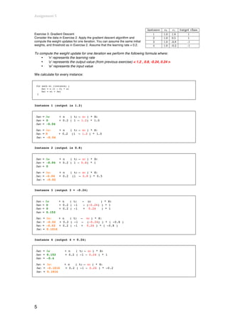
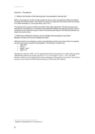
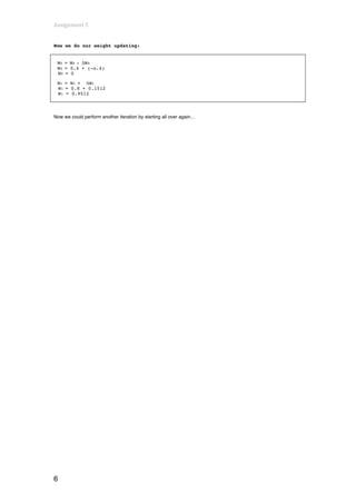
The document discusses perceptrons and gradient descent algorithms for training perceptrons on classification tasks. It contains 4 exercises: 1) Explains the role of the learning rate in perceptron training and which Boolean functions can/cannot be modeled with perceptrons. 2) Applies a perceptron to a sample dataset, calculates outputs, and determines the accuracy. 3) Performs one iteration of gradient descent on the same dataset, computing weight updates with a learning rate of 0.2. 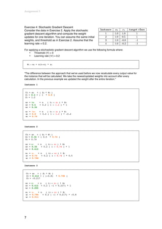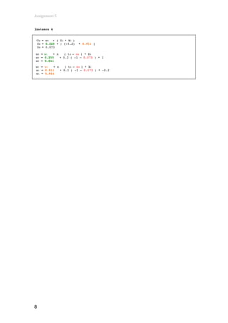4) Performs one iteration of stochastic gradient descent on the dataset, recomputing outputs and updating weights after each instance.

1. Data mining
Assignment week 5
BARRY KOLLEE
10349863

2. Assignment
5
Exercise 1: Perceptrons
1.1 What is the function of the learning rate in the perceptron training rule?
Within our perceptrons we take a certain weight into account when calculating the difference between
the target and outcome values. This weight it’s purpose is to adjust the actual value which we compare
to a certain threshold (i.e. ‘do we play tennis; yes or no?’).
The learning rate it’s goal is to define the extend of this weight adjustment. This learning rate can be
described as a sensitivity for our calculation of the difference between the target and outcome value. In
conclusion we can state that we give a value to this learning rate based on the difference between the
target and outcome value.
1.2 What kind of Boolean functions can be modeled with perceptrons and which
Boolean functions can not be modeled and why?
Within the model of our perceptron we take several Boolean functions into account which we regularly
see within the common programming languages. These Boolean conditions are:
• AND (‘&&’)
• OR (‘||’)
• NAND (‘! &&’)
• NOR (‘! ||’)
The Boolean condition ‘XOR’ can’t be implemented within the perceptron it’s model. When using the
XOR Boolean function the output can only be 1 if x1 is not equal to x2 (x1 != x2)1. The XOR
Boolean condition can be represented by using combinations of perceptrons (more then 1-level) That’s
because we can express the XOR statement using an AND and an OR condition.
1
Objective C representation of x1 not equal to x2
2

3. Assignment
5
Exercise 2: Weight Updating in Perceptrons
Assume the following set of instances with the weights: w0 = 0.4 and w1 = 0.8. The threshold
is 0.
What are the output values for each instance
before the threshold function is applied? What is
the accuracy of the model when applying the
threshold function?
For calculating the output values of the instances we perform the following formula:
Instance value = w0 + (x1 * w1)
Output value:
1 if((w0 + (x1 * w1) +… +(xn * wn))) > 0
-1 otherwise
With these formula’s we can find the output values of every instance within the table. If the result of the
instance value is higher then 0 the output value is 1. If this is not the case we set it to -1. Underneath are
all formula results and output values. They formula results are given in green and the output values are
in red.
Instance 1 :
Instance 1 = 0.4 + (0.8 * 1.0)
Instance 1 = 0.4 + 0.8
Instance 1 = 1.2
Instance 1 > threshold
Output value for instance 1 = 1.0
Instance 2 :
Instance 2 = 0.4 + (0.8 * 0.5)
Instance 2 = 0.4 + 0.4
Instance 2 = 0.8
Instance 2 > threshold
Output value for instance 2 = 1.0
Instance 3:
Instance 3 = 0.4 + (0.8 * -0.8)
Instance 3 = 0.4 - 0.64
Instance 3 = -0.24
Instance 3 < threshold
Output value for instance 3 = -1.0
3

4. Assignment
5
Instance 4:
Instance 4 = 0.4 + (0.8 * 1.0) + (0.8 * -0.2)
Instance 4 = 0.4 - 0.16
Instance 4 = 0.24
Instance 4 > threshold
Output value for instance 4 = 1.0
If we compare these output values with the instance it’s Instance Target Output
target value. We can state that we have a 75 % accuracy class value
th
because ¾ of the target classes is equal to it’s respective value
output value.
1 1 1
2 1 1
3 -1 -1
4 -1 1
4

5. Assignment
5
Exercise 3: Gradient Descent
Consider the data in Exercise 2. Apply the gradient descent algorithm and
compute the weight updates for one iteration. You can assume the same initial
weights, and threshold as in Exercise 2. Assume that the learning rate = 0.2.
To compute the weight update for one iteration we perform the following formula where:
• ‘n’ represents the learning rate
• ‘o’ represents the output value (from previous exercise) < 1.2 , 0.8, -0.24, 0.24 >
• ‘xi’ represents the input value
We calculate for every instance:
for each wi (instance) {
Δwi = n (t – 0) * xi
Δwi = wi + Δwi
}
Instance 1 (output is 1.2)
Δw0 = Δw + n ( t2 – o2 ) * X0
Δw0 = 0 + 0.2 ( 1 – 1.2) * 1.0
Δw0 = -0.04
Δw1 = Δw1 + n ( t2 – o2 ) * X1
Δw1 = 0 + 0.2 (1 – 1.2 ) * 1.0
Δw1 = -0.04
Instance 2 (output is 0.8)
Δw0 = Δw + n ( t2 – o2 ) * X0
Δw0 = -0.04 + 0.2 ( 1 - 0.8) * 1
Δw0 = 0
Δw1 = Δw1 + n ( t2 – o2 ) * X1
Δw1 = -0.04 + 0.2 (1 – 0.8 ) * 0.5
Δw1 = -0.02
Instance 3 (output 3 = -0.24)
Δw0 = Δw + n ( t2 - o2 ) * X0
Δw0 = 0 + 0.2 ( -1 - (-0.24) ) * 1
Δw0 = 0 + 0.2 ( -1 + 0.24 ) * 1
Δw0 = 0.152
Δw1 = Δw1 + n ( t2 – o2 ) * X1
Δw1 = -0.02 + 0.2 ( -1 – (-0.24) ) * ( -0.8 )
Δw1 = -0.02 + 0.2 ( -1 + 0.24 ) * ( -0.8 )
Δw1 = 0.1016
Instance 4 (output 4 = 0.24)
Δw0 = Δw + n ( t2 – o2 ) * X0
Δw0 = 0.152 + 0.2 ( -1 - 0.24 ) * 1
Δw0 = -0.4
Δw1 = Δw1 + n ( t2 – o2 ) * X1
Δw1 = -0.1016 + 0.2 ( -1 - 0.24 ) * -0.2
Δw1 = 0.1016
5

6. Assignment
5
Now we do our weight updating:
W0 = W0 + ΔW0
W0 = 0.4 + (-o.4)
W0 = 0
W1 = W1 + ΔW1
W1 = 0.8 + 0.1512
W1 = 0.9512
Now we could perform another iteration by starting all over again…
6

7. Assignment
5
Exercise 4: Stochastic Gradient Descent
Consider the data in Exercise 2. Apply the stochastic
gradient descent algorithm and compute the weight
updates for one iteration. You can assume the same initial
weights, and threshold as in Exercise 2. Assume that the
learning rate = 0.2.
For applying a stochastistic gradient descent algorithm we use the following formula where:
• Threshold (‘t’) = 0
• Learning rate (‘n’) = 0.2
Wi = wi + n(t-o) * xi
“The difference between the approach that we've used before we now recalculate every output value for
the instance that will be calculated. We take the newest/updated weights into account after every
calculation. In the previous example we updated the weight after the entire iteration.”
Instance 1
O1 = w0 + ( X1 * W1 )
O1 = 0.4 + ( 1 * 0.8 )
O1 = 1.2
w0 = Δw + n ( t1 – o1 ) * X0
w0 = 0.4 + 0.2 ( 1 – 1.2 ) * 1
w0 = 0.36
w1 = Δw1 + n ( t1 – o1 ) * X1
w1 = 0.8 + 0.2 ( 1 – 1.2 ) * -0.2
w1 = 0.76
Instance 2
O2 = w0 + ( X1 * W1 )
O2 = 0.36 + ( 0.5 * 0.76 )
O2 = 0.74
w0 = w1 + n ( t2 – o2 ) * X0
w0 = 0.36 + 0.2 ( 1 – 0.74 ) * 1
w0 = 0.412
w1 = w1 + n ( t2 – o2 ) * X1
w1 = 0.76 + 0.2 ( 1 – 0.74 ) * 0.5
w1 = 0.786
Instance 3
O3 = w0 + ( X1 * W1 )
O3 = 0.412 + ( (-0.8) * 0.786 )
O3 = -0.217
w0 = w1 + n ( t3 – o3 ) * X0
w0 = 0.412 + 0.2 ( -1 + 0.217) * 1
w0 = 0.255
w1 = w1 + n ( t3 – o3 ) * X1
w1 = 0.786 + 0.2 ( -1 + 0.217) * -0.8
w1 = 0.911
7

8. Assignment
5
Instance 4
O4 = w0 + ( X1 * W1 )
O4 = 0.225 + ( (-0.2) * 0.911 )
O4 = 0.073
w0 = w1 + n ( t4 – o4 ) * X0
w0 = 0.255 + 0.2 ( -1 – 0.073 ) * 1
w0 = 0.041
w1 = w1 + n ( t4 – o4 ) * X1
w1 = 0.911 + 0.2 ( -1 – 0.073 ) * -0.2
w1 = 0.954
8