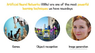
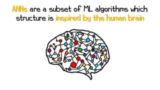
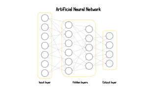
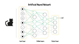
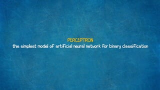
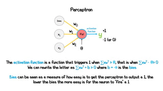
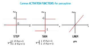
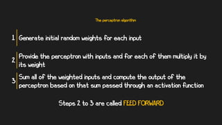
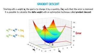
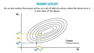
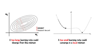
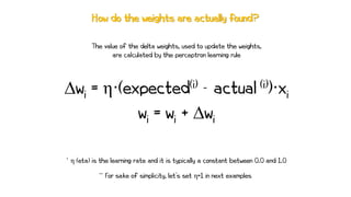
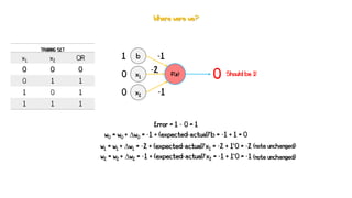
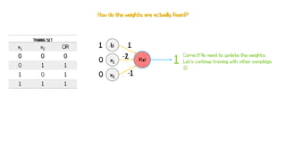
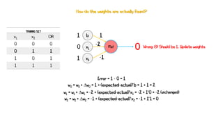
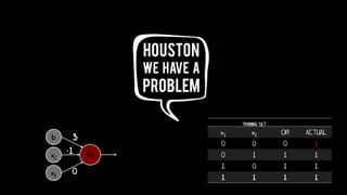
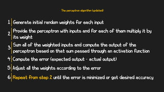
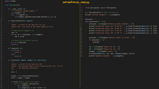
Artificial neural networks (ANNs) are a subset of machine learning algorithms inspired by the human brain. ANNs consist of interconnected artificial neurons that can learn complex patterns from data. The document introduces ANNs and perceptrons, the simplest type of ANN for binary classification. It discusses how perceptrons use weighted inputs and an activation function to make predictions. The perceptron learning rule is then explained, showing how weights are updated during training to minimize errors by calculating delta weights through gradient descent. This allows perceptrons to learn logical functions like AND, OR, and NOT from examples.

1. ARTIFICIAL
NEURAL NETWORKS
INTRODUCTION TO
Damian A. Tamburri Stefano Dalla Palma Daniel De Pascale

2. Object recognition
Games Image generation
Artificial Neural Networks (ANNs) are one of the most powerful
learning techniques we have nowadays
https://thispersondoesnotexist.com

3. ANNs are a subset of ML algorithms which
structure is inspired by the human brain

4. INPUT STRENGTHS TRANSFORM OUTPUT
axone synaptic terminal
dentrites cell body
SUM
Biological Neuron

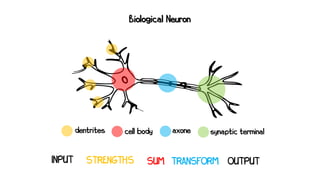
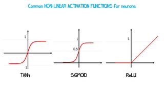
5. Artificial Neuron
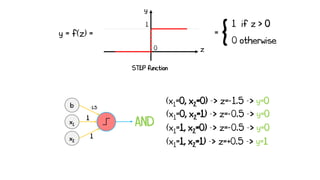
y = f(x·wT + b)
x = [x0, x1, …, x3] w = [w0, w1, …, wn]
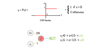
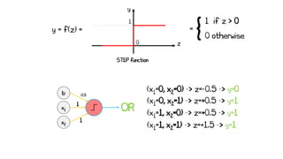
If f(z) > θ then the neuron is activated and the signal is propagated
x0
f(z)
x1
xn
w0
w1
wn
…
θthreshold
activation
function
y
input
input
input
weights

6. Artificial Neural Network
Input layer Hidden layers Output layer

7. Artificial Neural Network
…
Input layer Hidden layers Output layer
CAT

8. PERCEPTRON
the simplest model of artificial neural network for binary classification

9. Perceptron
activation
function
x1
f(z)
x2
w0
w2
+1
-1 (or 0)
θ
y
bias
w1
Bias can be seen as a measure of how easy is to get the perceptron to output a 1, the
lower the bias the more easy is for the neuron to “fire” a 1
The activation function is a function that triggers 1 when ∑xwT > θ, that is when ∑xwT - θ> 0
We can rewrite the latter as ∑xwT + b > 0 where b = -θ is the bias

10. Common ACTIVATION FUNCTIONS for perceptron
+1
STEP
y ={1 If f(z) > 0
0 if f(z) <= 0
+1
-1
SIGN
y ={ 1 If f(z) > 0
-1 if f(z) <= 0
f(z)
z z
f(z)
y=x
LINER
z
f(z)
0

11. The perceptron algorithm
Generate initial random weights for each input
1
Provide the perceptron with inputs and for each of them multiply it by
its weight
2
Sum all of the weighted inputs and compute the output of the
perceptron based on that sum passed through an activation function
3
Steps 2 to 3 are called FEED FORWARD

12. perceptron.py main.py
TERMINAL

13. Neural representation of the logical complement (NOT)
Unary connective that return 0 if the operand is 1, and 1 if the operand is 0
x1 NOT
0 1
1 0
x1
f(z)
w1
NOT
bias w0
θ

14. x1
-1
NOT
bias 0.5
x1=0 -> z=0.5 -> y=1
x1=1 -> z=-0.5 -> y=0
1
0 z
y
{
1 if z > 0
0 otherwise
=
y = f(z) =
STEP function

15. Neural representation of the inclusive disjunction (OR)
A bitwise operator that yields 1 when any of its operands is 1
x1 x2 OR
0 0 0
0 1 1
1 0 1
1 1 1
f(z) OR
w0
θ
x2
x1
b
w1
w2

16. 1
0 z
y
{
1 if z > 0
0 otherwise
=
y = f(z) =
STEP function
x2
OR
x1
1
(x1=0, x2=0) -> z=-0.5 -> y=0
(x1=0, x2=1) -> z=+0.5 -> y=1
(x1=1, x2=0) -> z=+0.5 -> y=1
(x1=1, x2=1) -> z=+1.5 -> y=1
b -0.5
1

17. Neural representation of the logical conjunction (AND)
A bitwise operator that yields 1 if and only if all operands are 1
x1 x2 AND
0 0 0
0 1 0
1 0 0
1 1 1
f(z) AND
w0
θ
x2
x1
b
w1
w2

18. x2
AND
x1
1
(x1=0, x2=0) -> z=-1.5 -> y=0
1
STEP function
0 z
y
{
1 if z > 0
0 otherwise
=
y = f(z) =
(x1=0, x2=1) -> z=-0.5 -> y=0
(x1=1, x2=0) -> z=-0.5 -> y=0
(x1=1, x2=1) -> z=+0.5 -> y=1
b -1.5
1

19. Neural representation of the negated
conjunction (NAND)
A bitwise operator that yields 0 if and only
if both operands are 1
x1 x2 NAND
0 0 ?
0 1 ?
1 0 ?
1 1 ?
Neural representation of the negated
inclusive disjunction (NOR)
A bitwise operator that yields 1 if and only
if both operands are 0
x1 x2 NOR
0 0 ?
0 1 ?
1 0 ?
1 1 ?

20. x1 x2 NAND
0 0 1
0 1 1
1 0 1
1 1 0
x1 x2 NOR
0 0 1
0 1 0
1 0 0
1 1 0
Neural representation of the negated
conjunction (NAND)
A bitwise operator that yields 0 if and only
if both operands are 1
Neural representation of the negated
inclusive disjunction (NOR)
A bitwise operator that yields 1 if and only
if both operands are 0

21. x2
NAND
x1
-1
(x1=0, x2=0) -> z=2 -> y=1
(x1=0, x2=1) -> z=1 -> y=1
(x1=1, x2=0) -> z=1 -> y=1
(x1=1, x2=1) -> z=0 -> y=0
b
-1
x2
NOR
x1
-1
(x1=0, x2=0) -> z=0.5 -> y=1
(x1=0, x2=1) -> z=-0.5 -> y=0
(x1=1, x2=0) -> z=-0.5 -> y=0
(x1=1, x2=1) -> z=-1.5 -> y=0
b
-1
2
0.5

22. How do the weights are actually found?
What if the initial random weights lead to wrong classifications?

23. How do the weights are actually found?
f(z)
OR
w0
x2
x1
b
w1
w2
TRAINNG SET
x1 x2 OR
0 0 0
0 1 1
1 0 1
1 1 1

24. f(z)
0
-1
x2
x1
b
-2
-1
1
0
0
Should be 1!
Error = expected output - actual output
Error = 1 - 0 = 1
How do the weights are actually found?

25. Imagine the following function that measure the total error for our
perceptron
𝒆𝒆𝒆𝒆𝒆𝒆𝒆𝒆𝒆𝒆 =
𝟏𝟏
𝟐𝟐
�
𝒊𝒊
𝒆𝒆𝒆𝒆𝒆𝒆𝒆𝒆𝒆𝒆𝒆𝒆𝒆𝒆𝒅𝒅𝒊𝒊
− 𝒂𝒂𝒂𝒂𝒂𝒂𝒂𝒂𝒂𝒂𝒍𝒍𝒊𝒊 𝟐𝟐
TRAINNG SET (OR)
i x1 x2 expected actual expectedi - actuali cumulative error
1 0 0 0 1 -1 1
2 0 1 1 0 1 2
3 1 0 1 0 1 3
4 1 1 1 0 1 4
Error = 2

26. Imagine the following function that measure the total error for our
perceptron
𝒆𝒆𝒆𝒆𝒆𝒆𝒆𝒆𝒆𝒆 =
𝟏𝟏
𝟐𝟐
�
𝒊𝒊
𝒆𝒆𝒆𝒆𝒆𝒆𝒆𝒆𝒆𝒆𝒆𝒆𝒆𝒆𝒅𝒅𝒊𝒊
− 𝒂𝒂𝒂𝒂𝒂𝒂𝒂𝒂𝒂𝒂𝒍𝒍𝒊𝒊 𝟐𝟐
TRAINNG SET (OR)
i x1 x2 expected actual expectedi - actuali cumulative error
1 0 0 0 0 0 0
2 0 1 1 1 0 0
3 1 0 1 1 0 0
4 1 1 1 1 0 0
Error = 0

27. Starting with a weight wi the goal is to change it by a quantity ∆wi such that the error is minimized
It is possible to calculate the delta weight with an optimization technique called gradient descent
GRADIENT DESCENT
w2
(B) = w2
(A) + ∆w2
w1
(B) = w1
(A) + ∆w1
Error
w1
w2

28. We can also visualize the previous surface as a set of elliptical contours, where the minimum error is
at the center of the ellipses
GRADIENT DESCENT
w2
w1
w2
(A)
w1
(A) w1
(B)
w2
(A)
∆w2
∆w1
GRADIENT
steepest descent

29. is called LEARNING RATE and tell us how
“fast” the weight must be updated
How large should be each step?
η

30. SMALL learning rate

31. HIGH learning rate

32. OPTIMAL learning rate

33. A too large learning rate could
diverge from the minimum
w2
w1
GRADIENT
steepest descent
A too small learning rate could
converge in a local minimum

34. ∆wi = η·(expected(i) - actual (i))·xi
How do the weights are actually found?
** For sake of simplicity, let’s set η=1 in next examples
wi = wi + ∆wi
The value of the delta weights, used to update the weights,
are calculated by the perceptron learning rule
* η (eta) is the learning rate and it is typically a constant between 0.0 and 1.0

35. f(z)
0
-1
x2
x1
b
-2
1
0
0
Should be 1!
Error = 1 - 0 = 1
Where were we?
w0 = w0 + ∆w0 = -1 + (expected-actual)*b = -1 + 1 = 0
w1 = w1 + ∆w1 = -2 + (expected-actual)*x1 = -2 + 1*0 = -2
w2 = w2 + ∆w2 = -1 + (expected-actual)*x2 = -1 + 1*0 = -1
(note unchanged)
TRAINNG SET
x1 x2 OR
0 0 0
0 1 1
1 0 1
1 1 1
-1
(note unchanged)

36. f(z)
0
0
x2
x1
b
-2
1
0
0
Should be 1!
Error = 1 - 0 = 1
Where were we?
w0 = w0 + ∆w0 = 0 + (expected-actual)*b = 0 + 1 = 1
w1 = w1 + ∆w1 = -2 + (expected-actual)*x1 = -2 + 1*0 = -2
w2 = w2 + ∆w2 = -1 + (expected-actual)*x2 = -1 + 1*0 = -1
(note unchanged)
TRAINNG SET
x1 x2 OR
0 0 0
0 1 1
1 0 1
1 1 1
-1
(note unchanged)

37. f(z)
1
1
x2
x1
b
-2
-1
1
0
0
How do the weights are actually found?
TRAINNG SET
x1 x2 OR
0 0 0
0 1 1
1 0 1
1 1 1
Correct! No need to update the weights.
Let’s continue training with other samplings


38. f(z)
0
1
x2
x1
b
-2
-1
1
0
1
How do the weights are actually found?
TRAINNG SET
x1 x2 OR
0 0 0
0 1 1
1 0 1
1 1 1
Wrong ! Should be 1. Update weights
Error = 1 - 0 = 1
w0 = w0 + ∆w0 = 1 + (expected-actual)*b = 1 + 1 = 2
w1 = w1 + ∆w1 = -2 + (expected-actual)*x1 = -2 + 1*0 = -2
w2 = w2 + ∆w2 = -1 + (expected-actual)*x2 = -1 + 1*1 = 0
(unchanged)

39. f(z)
1
2
x2
x1
b
-2
0
1
0
1
How do the weights are actually found?
TRAINNG SET
x1 x2 OR
0 0 0
0 1 1
1 0 1
1 1 1
Correct! No need to update the weights.
Let’s continue training with other samplings


40. f(z)
0
2
x2
x1
b
-2
0
1
1
0
How do the weights are actually found?
TRAINNG SET
x1 x2 OR
0 0 0
0 1 1
1 0 1
1 1 1
Wrong ! Should be 1. Update weights
Error = 1 - 0 = 1
w0 = w0 + ∆w0 = 2 + (expected-actual)*b = 2 + 1 = 3
w1 = w1 + ∆w1 = -2 + (expected-actual)*x1 = -2 + 1*1 = -1
w2 = w2 + ∆w2 = 0 + (expected-actual)*x2 = 0 + 1*0 = 0 (unchanged)

41. f(z)
1
3
x2
x1
b
-1
0
1
1
0
How do the weights are actually found?
TRAINNG SET
x1 x2 OR
0 0 0
0 1 1
1 0 1
1 1 1
Correct! No need to update the weights.
Let’s continue training with other samplings


42. f(z)
1
3
x2
x1
b
-1
0
1
1
1
How do the weights are actually found?
TRAINNG SET
x1 x2 OR
0 0 0
0 1 1
1 0 1
1 1 1
Correct! No need to update the weights.
Let’s continue training with other samplings


43. f(z)
3
x2
x1
b
-1
0
TRAINNG SET
x1 x2 OR ACTUAL
0 0 0 1
0 1 1 1
1 0 1 1
1 1 1 1

44. Repeat the previous steps with more training data,
but let’s automate it 

45. The perceptron algorithm (updated)
Generate initial random weights for each input
1
Provide the perceptron with inputs and for each of them multiply it by
its weight
2
Sum all of the weighted inputs and compute the output of the
perceptron based on that sum passed through an activation function
3
Compute the error (expected output - actual output)
4
Adjust all the weights according to the error
5
Repeat from step 2 until the error is minimized or got desired accuracy
6

46. perceptron.py main.py

47. If training data is linearly separable
PRECEPTRON
CONVERGENCE THEOREM
Learning rate is sufficiently small
AND
THEN
The perceptron training will converge towards solution*
*Means the perceptron will stop updating their weights after a finite number of steps

48. Neural representation of the exclusive disjunction (XOR)
A bitwise operator that yields 1 when one of its operands is 1, not both
x1 x2 XOR
0 0 0
0 1 1
1 0 1
1 1 0
Can you catch the problem?

49. 1
1
0
1
1
1
OR
1
1
0
0
0
1
AND
1
1
1
1
1
0
NAND
1
1
1
0
0
0
NOR
1
1
0
1
1
0
XOR

50. Neural representation of the exclusive disjunction (XOR)
x1 x2 XOR ? ?
0 0 0 1 0
0 1 1 1 1
1 0 1 1 1
1 1 0 0 1
Remember these?

51. 1
1
0
1
1
1
OR
1
1
0
0
0
1
AND
1
1
1
1
1
0
NAND
1
1
1
0
0
0
NOR
1
1
0
1
1
0
XOR

52. 1
1
0
1
1
1
OR
1
1
1
1
0
NAND
1
1
0
1
1
0
XOR

53. x1 x2 XOR NAND OR
0 0 0 1 0
0 1 1 1 1
1 0 1 1 1
1 1 0 0 1
Which operator to use to combine NAND and OR to get the XOR?
Neural representation of the exclusive disjunction (XOR)
1
1
0
1
1
1
OR
1
1
1
1
0
NAND
1
1
0
1
1
0
XOR

54. x2
XOR
x1
1
b1
-0.5
1
-1
-1
2
y1 [OR]
1
1
b2
-1.5
y2 [NAND]
y3 [AND]

55. x2
0
x1
1
b1
-0.5
1
-1
-1
2
y2 [NAND]
y1 [OR]
y3 [AND]
1
1
b2
-1.5
x1 = 0 x2 = 0
Neuron activated - “Fires” 1
Neuron not activated - “Fires” 0
z1 = -0.5 -> y1 = 0
z2 = 2 -> y2 = 1
z3 = -0.5 -> y3 = 0
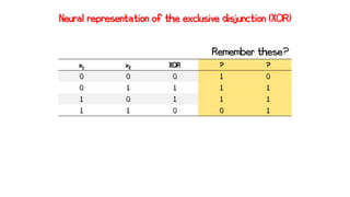
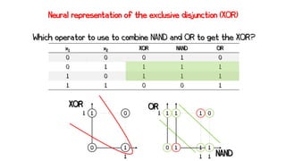
x1 x2 XOR
0 0 0

56. x2
1
x1
1
b1
-0.5
1
-1
-1
2
y2 [NAND]
y1 [OR]
y3 [AND]
1
1
b2
-1.5
x1 = 0 x2 = 1
Neuron activated - “Fires” 1
Neuron not activated - “Fires” 0
z1 = 0.5 -> y1 = 1
z2 = 0.5 -> y2 = 1
z3 = 0.5 -> y3 = 1
x1 x2 XOR
0 0 0
0 1 1

57. x2
1
x1
1
b1
-0.5
1
-1
-1
2
y2 [NAND]
y1 [OR]
y3 [AND]
1
1
b2
-1.5
x1 = 1 x2 = 0
Neuron activated - “Fires” 1
Neuron not activated - “Fires” 0
z1 = 0.5 -> y1 = 1
z2 = 1 -> y2 = 1
z3 = 0.5 -> y3 = 1
x1 x2 XOR
0 0 0
0 1 1
1 0 1

58. x2
0
x1
1
b1
-0.5
1
-1
-1
2
y2 [NAND]
y1 [OR]
y3 [AND]
1
1
b2
-1.5
x1 = 1 x2 = 1
Neuron activated - “Fires” 1
Neuron not activated - “Fires” 0
z1 = 1.5 -> y1 = 1
z2 = 0 -> y2 = 0
z3 = -0.5 -> y3 = 0
x1 x2 XOR
0 0 0
0 1 1
1 0 1
1 1 0

59. SIGMOID
1
ReLU
TANh
0.5
1
1
-1
Common NON-LINEAR ACTIVATION FUNCTIONS for neurons