DWDM_UNIT4.pptx ddddddddddddddddddddddddddddd

Unit-IV Data Mining Introduction:
Basics of data mining, related concepts,
Data mining techniques Data Mining
Algorithms: Classification,
Clustering, Association rules. Knowledge
Discovery: KDD Process.

DATA MINING
INTRODUCTION
• Amount of data kept in the database is growing at a
phenomenal rate.
• Users of these data are expecting more sophisticated
information.
• A Marketing manager is no longer satisfied with a
simple listing of marketing contacts but wants detailed
information about customers past purchases as well
as predictions of future purchases.

• Simple structured /Query language queries are not
sufficient to support these increased demands for
information .
• Data mining solve these needs.
• Data mining is defined as finding hidden information
in a database, it is also called exploratory data
analysis, data driven discovery & Deductive learning.

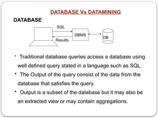
DATABASE Vs DATAMINING
DBMS
SQL
Results
DB
• Traditional database queries access a database using
well defined query stated in a language such as SQL.
• The Output of the query consist of the data from the
database that satisfies the query.
• Output is a subset of the database but it may also be
an extracted view or may contain aggregations.
DATABASE

DATA MINING
Data mining access of a database differs from traditional access
Query :
• The query might not be well formed or precisely stated .
• The data miner might not be exactly sure of what he wants to see.
Data :
• The data accessed is usually a different version from that of the
original operational database.
• The data have been cleansed and modified to better support the
mining process
Output :
• The output of the data mining query probably is not a subset of the
database.
• Output is some analysis of the contents of the database

Ex :Credit card companies must determine whether to
authorize credit card purchases .Suppose that based on
past historical information about purchases ,each
purchase is placed into one of four classes 1)Authorize
2)ask for further identification before authorization 3)Do
not authorize and 4)Do not authorize but contact police.
Data mining functions are two fold
1.Historical data must be examined to determine how
the data fit into the four classes. Then the problem is to
apply this model to each new purchase.
2.The second part indeed stated as a simple database
query. the first part can not be.

DATA MINING :Definitions
1. Data mining or knowledge discovery in databases ,as it
is also known, is the non trivial extraction of
implicit ,previously unknown and potentially useful
information from the data. This encompasses a number of
technical approaches such as clustering ,data
summarization ,classification ,finding dependency
networks ,analyzing changes and detecting anomalies.
2.Datamining is the search for the relationships and global
patterns that exist in large databases but are hidden
among vast amounts of data, such as the relationship
between patient data and their medical diagnosis .This
relationship represents valuable knowledge about the
databases ,and the objects in the database, if the
database is a faithful mirror of the real world.

3.Data mining refers to using a variety of techniques to
identify nuggets of information or decision making
knowledge in the database and extracting these in such
a way that they can be put to use in areas such as
decision support, prediction, forecasting and
estimation .the data is often voluminous ,but it has low
value and no direct use can be made of it .It is hidden
information in the data that is useful.
4.Data mining is the process of discovering
meaningful ,new correlation patterns and trends by
sifting through large amount of data stored in
repositories ,using pattern recognition techniques as
well as statistical and mathematical techniques.

5.Discovering relations that connect variables in a
database is the subject of data mining .The data mining
system self learns from the previous history of the
investigated system, formulating and testing hypothesis
about rules which systems obey. When concise and
valuable knowledge about the system of interest is
discovered ,it can and should be interpreted into some
decision support system, which help the manager to
make wise and informed business decisions

• Data mining involves different algorithms to accomplish
different tasks.
• These algorithm attempt to fit a model to the data.
• The algorithm examine the data and determine a model
that is closest to the characteristics of the data being
examined
Data mining algorithm can be characterized as consisting of
three parts
Model: The purpose of the algorithm is to fit a model to the
data
Preference: some criteria must be used to fit one model over
another.
Search :All algorithms require some technique to search the
data

Data Mining Models and Tasks
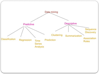
Predictive Model:
• This model makes prediction about values of data using
known results found from different data.
• Predictive modeling may be made based on the use of
historical data.
• Predictive model data mining tasks include classification
,regression ,time series analysis and prediction.

Descriptive Model
• A descriptive model identifies patterns or relationships in
data.
• Descriptive model serves as a way to explore the
properties
of the data examined ,not to predict new properties.
• Descriptive model data mining task includes Clustering
,summarization, association rules and sequence discovery

Data mining
Predictive Descriptive
Classification Regression Time
Series
Analysis
Prediction
Clustering Summarization
Association
Rules
Sequence
Discovery

Basic Data Mining Tasks
Classification:
• Classification maps data into predefined groups or classes.
• It is referred to as supervised learning because the classes are
determined before examining the data.
• Classification algorithm require that the classes be defined based
on data attribute values.
• They describe classes looking at the characteristics of data
already known to belong to the classes.
• Pattern recognition is a type of classification where an input
pattern is classified into one of several classes based on its
similarity to these predefined classes

Regression:
• Regression is used to map a data item to a real valued
prediction variable.
• Regression involves the learning of the function that
does this mapping
• It assumes that the target data fit into some known
type
of function (e.g linear, logistic etc.) and determines the
best function of this type that models the given data.
• Some type of error analysis is used to determine which
function is best

Time Series Analysis :
• With time series analysis ,the value of attribute is examined
as it varies over time.
• The values usually are obtained as evenly spaced time
points( daily, weekly, hourly, etc)
• A time series plot is used to visualize the time series.
• Three functions performed in time series analysis
 Distance measures are used to determine the similarity
between different time series
 The structure of the line is examined to determine its behavior.
 Historical time series plot is used to predict future values.

Prediction :
• Many data mining applications can be seen as predicting future data
states based on past and current data.
• Prediction can be viewed as a type of classification.
• Prediction is predicting a future state rather than a current state.
• Prediction application include flooding, speech recognition, machine
learning and pattern recognition.
• Future values may be predicted using time series analysis or
regression technique

Clustering :
• Clustering is similar to classification except that the groups are not
predefined but rather defined by the data alone.
• It is referred as unsupervised learning or segmentation.
• It is partitioning or segmenting the data into groups that might or
might not be disjoint.
• Clustering is usually accomplished by determining the similarity
among the data on predefined attributes.
• Clusters are not predefined ,a domain expert is required to interpret
the meaning of the created clusters.
• A special type of clustering is called segmentation. With
segmentation a database is partitioned into disjointed grouping of
similar tuples called segments. Segmentation is being viewed as
identical to clustering.

Summarization :
• Summarization maps data into subsets with associated simple
descriptions.
• It is also called characterization or generalization.
• It extracts or derives representative information about the
database.
• This is accomplished by actually retrieving portions of the data and
summary type information (mean of some numeric attribute)
is derived from the data.

Association Rules :
• Association refers to the data mining task of finding the
relationships among data referred as link analysis or affinity
analysis.
• An association rule is a model that identifies specific type of data
associations.
• Users of association rules must be cautioned that these are not
causal relationships. they do not represent any relationship
inherent in the actual data (functional dependencies) or in the
real world.
• Association rules can be used to assist retail store management
in effective advertising ,marketing and inventory control.

Sequence Discovery :
• Sequence Discovery is used to determine sequential patterns in
data also referred as Sequence analysis.
• These patterns are based on time sequence of actions.
• These patterns are similar to association but relationship is
based
on time.
• In Market basket analysis the items to be purchased at the same
time ,in sequence discovery the items are purchased over time in
some order.

DATA MINING VERSUS KNOWLEDGE DISCOVERY IN
DATABASES
Knowledge Discovery in Databases and Data Mining
are used interchangeably .The other name given to this
process of discovering useful (hidden) patterns in data
are knowledge extraction ,Information
discovery ,exploratory data analysis, information
harvesting and unsupervised pattern recognition..
KDD has been used to refer to a process consisting of
many steps while data mining is only one of these
steps.

Knowledge Discovery in Databases is the process of
identifying a valid, potentially useful and ultimately
understandable structure in data .This process involves
selecting or sampling data from data warehouse, cleaning
or preprocessing it, transforming or reducing it, applying a
data mining component to produce a structure and then
evaluating the derived structure.
Data mining is a step in the KDD process concerned with
the algorithmic means by which patterns or structures are
enumerated from the data under acceptable computational
efficiency limitations.
The structures that are outcome of the data mining process
must meet certain conditions so that these can be
considered as knowledge .these conditions are
validity ,understandability, utility and novelty.

Stages Of KDD :
KDD is a process that involves many different steps. The input to this
process is the data and the output is the useful information desired by
the users. objective is unclear or inexact .process itself is interactive
and require much elapsed time.
Selection :
• The data needed for the data mining process may be obtained from
many different and heterogeneous data sources.
• This step obtains the data from various databases ,files and
non electronic sources.
Preprocessing :
• The data to be used by the process may have incorrect or missing
data.
• There may be anomalous data from multiple sources involving
different data types and metrics.

• Erroneous data may be corrected or removed , whereas missing data
must be supplied or predicted.
Transformation :
• Data from different sources must be converted into a common format
for processing.
• Some data may be encoded or transformed into more usable formats.
• Data Reduction may be used to reduce number of possible data
values
being considered.
Transformation techniques are used to make the data easier to mine and
more useful to provide more meaningful results.

• The actual distribution of data modified to facilitate use by technique
that require specific types of data distribution.
• Some attributes may be combined to provide new values reducing
complexity of data.
• Real valued attributes may be more easily handled by partitioning the
values into ranges and using these discrete range values.
• Remove Outliers ,these are values that occur infrequently.
• A common transformation function is to use the log of the values rather
than value itself.
Data Mining :
• Based on the data mining task being performed ,This step applies
algorithms to the transformed data to generate the desired results.

Interpretation and Evaluation :
• The patterns obtained in the data mining stage are converted into
knowledge ,which in turn is used to support decision making.
Data Visualization :
• How the data mining results are presented to the users is extremely
important because usefulness of the results is dependent on it.
• Various visualization and GUI strategies are used at this last stage.
• Visualization refers to the visual presentation of the data.
Visual Techniques
Graphical :
• Traditional graph structures including bar charts, pie charts,
histograms, and the line graph may be used

Geometric :
• Geometric techniques include the box plot and scatter diagram technique.
Icon-based :
• Using figures ,colors or other icons can improve the presentation of the
results.
Pixel-based :
• With these techniques each data value is shown as a uniquely colored
pixel.
Hierarchical :
• These technique hierarchically divide the display area (screen) into
regions
based on data values.
Hybrid :
• The preceding approaches can be combined into one display.

How Database Is Used In Data Mining
There are three different ways in which data mining system use a
relational DBMS.
Database may not use at all :
• Data mining system do not use any DBMS and have their own
memory and storage management.
• They treat database simply as a data repository from which data is
expected to be down loaded into their own memory structures before
data mining algorithm starts.
• Advantage is one can optimize memory management specific to the
data mining algorithm
• These system ignore the field proven technologies of DBMS such
as
recovery, concurrency.

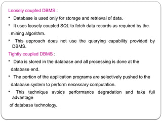
Loosely coupled DBMS :
• Database is used only for storage and retrieval of data.
• It uses loosely coupled SQL to fetch data records as required by the
mining algorithm.
• This approach does not use the querying capability provided by
DBMS.
Tightly coupled DBMS :
• Data is stored in the database and all processing is done at the
database end.
• The portion of the application programs are selectively pushed to the
database system to perform necessary computation.
• This technique avoids performance degradation and take full
advantage
of database technology.

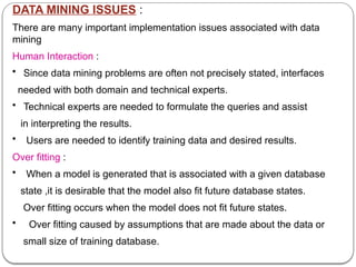
DATA MINING ISSUES :
There are many important implementation issues associated with data
mining
Human Interaction :
• Since data mining problems are often not precisely stated, interfaces
needed with both domain and technical experts.
• Technical experts are needed to formulate the queries and assist
in interpreting the results.
• Users are needed to identify training data and desired results.
Over fitting :
• When a model is generated that is associated with a given database
state ,it is desirable that the model also fit future database states.
Over fitting occurs when the model does not fit future states.
• Over fitting caused by assumptions that are made about the data or
small size of training database.

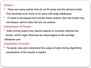
Outliers :
• There are many entries that do not fit nicely into the derived model.
This becomes even more of an issue with large databases.
• If model is developed that include these outliers, then the model may
not behave well for data that are not outliers.
Interpretation of Results :
• Data mining output may require experts to correctly interpret the
results, which might otherwise be meaningless to the average
database user.
Visualization of results:
• To easily view and understand the output of data mining algorithms
,visualization of the results is helpful.

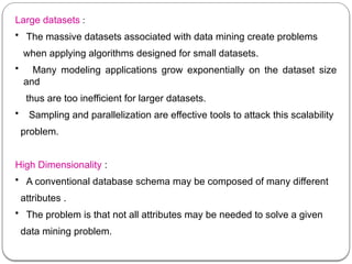
Large datasets :
• The massive datasets associated with data mining create problems
when applying algorithms designed for small datasets.
• Many modeling applications grow exponentially on the dataset size
and
thus are too inefficient for larger datasets.
• Sampling and parallelization are effective tools to attack this scalability
problem.
High Dimensionality :
• A conventional database schema may be composed of many different
attributes .
• The problem is that not all attributes may be needed to solve a given
data mining problem.

High Dimensionality :
• The use of other attributes may simply increase the overall
complexity and decrease the efficiency of an algorithm .
This problem is referred as Dimensionality Curse. meaning that
there are many attributes (dimensions) involved and it is difficult to
determine which one should be used .one solution to this high
dimensionality problem is to reduce the number of attributes,
which is known as Dimensionality Reduction.
Multimedia Data :
• Previous data mining algorithms are targeted to traditional data
types (numeric,character,text etc).
• The use of multimedia data found in GIS databases
complicates or invalidates many proposed algorithms.

Missing Data :
• During the preprocessing phase of KDD ,missing data may be replaced
with estimates.
• Missing data can lead to invalid results in the data mining steps.
Irrelevant Data :
• Some attributes in the database might not be of interest to the data
mining task being developed.
Noisy Data :
• Some attributes values might be invalid or incorrect. These values are
often corrected before running data mining applications

Changing Data :
• Databases can not be assumed to be static.
• Most data mining algorithms do assume a static database.
• This requires that the algorithm be completely rerun anytime the
database change.
Integration :
• The KDD process is not currently integrated into normal data
processing activities.
• KDD requests may be treated as special, unusual or one-time needs.
This makes them inefficient ,ineffective and not general enough
to be used on an ongoing basis.
• Integration of data mining functions into DBMS systems
is certainly a desirable goal.

Application :
• Determining the intended use for the information obtained from the
data
mining function is a challenge.
• How business executives effectively use the output is sometimes
considered the more difficult part, not running the algorithm themselves.
• Because Data are of type that has not previously been known,
business
practices may have to be modified to determine how to effectively use
the information uncovered.

DM Application Areas :
The discipline of data mining is driven in part by new applications which
require new capabilities that are not currently being supplied by today’s
technology.
These new applications can be naturally divided into two broad
categories.
A. BUSSINESS AND E-COMMERCE DATA
This is a major source category of data for data mining applications.
Back-office, front-office and network application produce large amount of
data about business processes .Using this data for effective decision
making remains a fundamental challenge.

BUSSINESS TRANSACTIONS
• Modern business processes are consolidating with millions of
customers
and billions of their transactions.
• Business enterprises requires necessary information for their effective
functioning in today’s competitive world.
Ex Information they want to know
“Is this transaction Fraud”,
”Which customer is likely to migrate”,
”What product is this customer most likely to buy next”
ELECTRONIC COMMERCE
Electronic commerce not only produce large data sets in which the
analysis of marketing patterns and risk patterns is critical but ,it is also
important to do this in near-real time to meet the demands of online
transactions.

B.SCIENTIFIC,ENGINEERING AND HEALTH CARE DATA
Scientific data and Metadata tend to be more complex in structure than
business data ,In addition ,scientists and engineers are making increasing
use of simulation and systems with application domain Knowledge.
GENOMIC DATA
Genomic sequencing and mapping efforts have produced a number of
databases which are accessible on the web. In addition ,there are also a
wide variety of other online databases. Finding relationships between
these data sources is another fundamental challenge for data mining.
SENSOR DATA
Remote sensing data is another source of voluminous data. Remote
satellites and a variety of other sensors produce large amount of
geo-referenced data. A fundamental challenge is to understand the
relationships ,including causal relationships amongst this data.

SIMULATION DATA
• Simulation is accepted as mode of science ,supplementing theory and
experiment. Today ,not only do experiments produce huge data sets ,but
so do simulations.
• Data mining is proving to be critical link between theory, simulation and
experiment.
HEALTH CARE DATA
• Hospitals ,health care organizations ,insurance companies and the
concerned government agencies accumulate large collections of data
about patients and health care related details
• Understanding relationships in this data is critical for a wide variety of
problems-ranging from determining what procedures and clinical
protocols are most effective, to how best deliver health care to the
maximum number of people.

WEB DATA
The data on the web is growing not only in volume but also in
complexity. Web data include text, audio and video material .
MULTIMEDIA DOCUMENTS
Today’s technology for retrieving multimedia items on the web is far
from satisfactory .on the other hand ,an increasingly large number
of matters on the web and the number of users is also growing
explosively. It is harder to extract meaningful information from the
archives of multimedia data as the volume grows.

DATA WEB
Today, the web is primarily oriented toward documents and their
multimedia extensions. HTML has proved itself to be a simple ,yet
powerful ,language for supporting this. Tomorrow, the potential
exists for the web to prove equally important for working with data in
networked environments. As this infrastructure grows, data mining is
expected to be a critical enabling technology for the emerging data
web

DATABASE/OLTP SYSTEMS
• A Database is a collection of data associated with some
organization
or enterprise.
• Data in database viewed to have a particular structure or schema
with which it is associated.
• Each record / tuple has a values associated for each of these
attributes.
• A Database is independent of the physical method used to store it
on Disk.
• A Database is also independent of the applications that access it.
• A Database Management System is the software to access a
database.

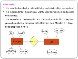
Data Model :
• It is used to describe the data, attributes and relationships among them.
• It is independent of the particular DBMS used to implement and access
the database.
• It is viewed as a documentation and communication tool to convey the
type and structure of the actual data. Common Data Model is E-R Data
model proposed in 1976.
Employee Job
Has Job
ID NAME
ADDRESS SALARY
Job Desc
Job No
Pay Range

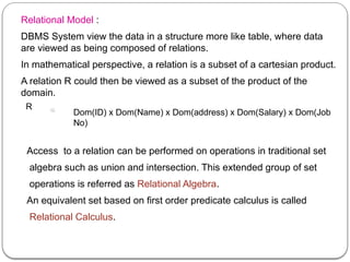
Relational Model :
DBMS System view the data in a structure more like table, where data
are viewed as being composed of relations.
In mathematical perspective, a relation is a subset of a cartesian product.
A relation R could then be viewed as a subset of the product of the
domain.
R
Dom(ID) x Dom(Name) x Dom(address) x Dom(Salary) x Dom(Job
No)
Access to a relation can be performed on operations in traditional set
algebra such as union and intersection. This extended group of set
operations is referred as Relational Algebra.
An equivalent set based on first order predicate calculus is called
Relational Calculus.

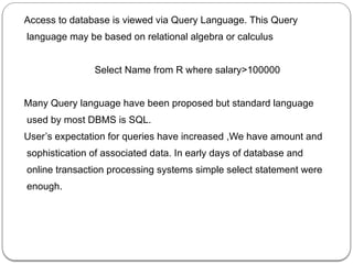
Access to database is viewed via Query Language. This Query
language may be based on relational algebra or calculus
Select Name from R where salary>100000
Many Query language have been proposed but standard language
used by most DBMS is SQL.
User’s expectation for queries have increased ,We have amount and
sophistication of associated data. In early days of database and
online transaction processing systems simple select statement were
enough.

FUZZY SETS AND FUZZY LOGIC : Lofty A Zadeh
Set : A Set is thought of as a collection of objects.
F={1,2,3,4,5}
Indicating set membership requirement F={x | x Є Z+
and x ≤ 5}
Fuzzy Set : Fuzzy Set is a set F in which set membership function F is
a real valued function with output in the range[0,1].
Membership value for kasturi being tall is 0.7 and value for her being
thin is 0.4.Membership value for her being both is 0.4 minimum of
both values .If these were really probabilities, product of these two
values has to be taken.

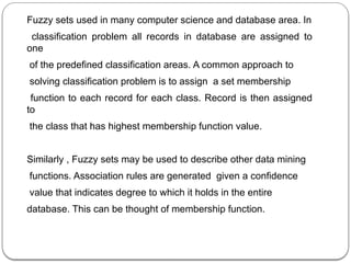
Fuzzy sets used in many computer science and database area. In
classification problem all records in database are assigned to
one
of the predefined classification areas. A common approach to
solving classification problem is to assign a set membership
function to each record for each class. Record is then assigned
to
the class that has highest membership function value.
Similarly , Fuzzy sets may be used to describe other data mining
functions. Association rules are generated given a confidence
value that indicates degree to which it holds in the entire
database. This can be thought of membership function.

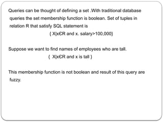
Queries can be thought of defining a set .With traditional database
queries the set membership function is boolean. Set of tuples in
relation R that satisfy SQL statement is
{ X|xЄR and x. salary>100,000}
Suppose we want to find names of employees who are tall.
{ X|xЄR and x is tall }
This membership function is not boolean and result of this query are
fuzzy.

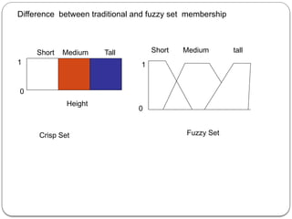
Difference between traditional and fuzzy set membership
Short Medium Tall
Height
Crisp Set
Short Medium tall
1
0
1
0
Fuzzy Set

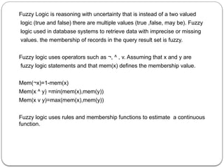
Fuzzy Logic is reasoning with uncertainty that is instead of a two valued
logic (true and false) there are multiple values (true ,false, may be). Fuzzy
logic used in database systems to retrieve data with imprecise or missing
values. the membership of records in the query result set is fuzzy.
Fuzzy logic uses operators such as ¬, ^ , v. Assuming that x and y are
fuzzy logic statements and that mem(x) defines the membership value.
Mem(¬x)=1-mem(x)
Mem(x ^ y) =min(mem(x),mem(y))
Mem(x v y)=max(mem(x),mem(y))
Fuzzy logic uses rules and membership functions to estimate a continuous
function.

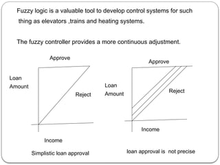
Fuzzy logic is a valuable tool to develop control systems for such
thing as elevators ,trains and heating systems.
The fuzzy controller provides a more continuous adjustment.
Approve
Loan
Amount
Reject
Income
Simplistic loan approval
Approve
Loan
Amount
Reject
Income
loan approval is not precise

INFORMATION RETRIEVAL
• It involves retrieving desired information from textual data.
• The historical development of IR was based on effective use of
libraries
so typical IR request is to find all library documents related to a
particular subject.
• In IR system documents are represented by document surrogates
consisting of data such as identifiers ,title ,author ,dates ,abstracts
,extracts ,reviews and keywords.
• As data consists of both formatted and unformatted (text) data ,
the retrieval of document is based on calculation of similarity
measure showing how close each document is to the desired result.
• An IR system consists of a set of documents D={D1,……Dn} ,the
input is query q stated as list of keywords .The similarity between
the query and each document is calculated Sim(q,Di).

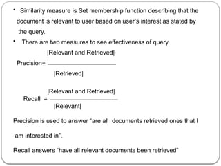
• Similarity measure is Set membership function describing that the
document is relevant to user based on user’s interest as stated by
the query.
• There are two measures to see effectiveness of query.
|Relevant and Retrieved|
Precision=
|Retrieved|
|Relevant and Retrieved|
Recall =
|Relevant|
Precision is used to answer “are all documents retrieved ones that I
am interested in”.
Recall answers “have all relevant documents been retrieved”

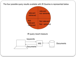
The four possible query results available with IR Queries is represented below
relevant
retrieved
Not
relevant
retrieved
relevant
not retrieved
Not relevant
Not retrieved
IR query result measure
IRS
Documents
Documents
keywords

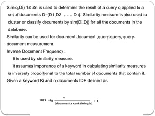
Sim(q,Di) 1≤ i≤n is used to determine the result of a query q applied to a
set of documents D={D1,D2,……..Dn}. Similarity measure is also used to
cluster or classify documents by sim(Di,Dj) for all the documents in the
database.
Similarity can be used for document-document ,query-query, query-
document measurement.
Inverse Document Frequency :
It is used by similarity measure.
it assumes importance of a keyword in calculating similarity measures
is inversely proportional to the total number of documents that contain it.
Given a keyword Ki and n documents IDF defined as

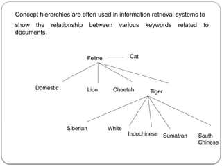
Concept hierarchies are often used in information retrieval systems to
show the relationship between various keywords related to
documents.
Feline Cat
Domestic Lion Cheetah Tiger
Siberian White
Indochinese Sumatran South
Chinese

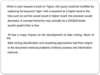
When a user request a book on Tigers ,this query could be modified by
replacing the keyword “tiger” with a keyword at a higher level in the
tree such as cat this would result in higher recall ,the precision would
decrease. A concept hierarchy may actually be a DAG(Directed
acyclic graph) than a tree.
IR has a major impact on the development of data mining. Much of
the
data mining classification and clustering approaches had their origins
in the document retrieval problems of library science and information
retrieval.

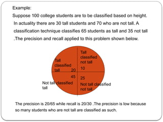
Example:
Suppose 100 college students are to be classified based on height.
In actuality there are 30 tall students and 70 who are not tall. A
classification technique classifies 65 students as tall and 35 not tall
.The precision and recall applied to this problem shown below.
Tall
classified
tall 20
45
Not tall classified
tall
Tall
classified
not tall
10
25
Not tall classified
not tall
The precision is 20/65 while recall is 20/30 .The precision is low because
so many students who are not tall are classified as such.

DECISION SUPPORT SYSTEM (DSS) ,EXECUTIVE INFORMATION
SYSTEM (EIS),EXECUTIVE SUPPORT SYSTEM (ESS):
• Decision Support System are comprehensive computer systems and
related tools that assist managers in making decisions and solving
problem.
• The goal is to improve the decision making process by providing
specific
information needed by the management.
• These system differ from traditional database management system in
that more adhoc queries and customized information is provided.
• EIS and ESS aim at developing the business structure and computer
technique to better provide information needed by the management to
make effective business decision.

• Data mining thought of as a suite of tools that assist in overall DSS
process
• A Decision support system is enterprise wide ,thus allowing upper
level managers the data needed to make intelligent business decision
that impact entire company.
• A DSS operates using Data warehouse data. alternatively A DSS
could be built around single user and PC.
DSS gives managers the tools needed to make intelligent
Decisions.

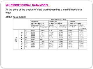
MULTIDIMENSIONAL DATA MODEL:
At the core of the design of data warehouse lies a multidimensional
view
of the data model
Professional Class
Engineer Secretary Teacher
PROFESSION PROFESSION PROFESSION
Chemical
Engineer
Civil
Engineer
Junior
Secretary
Executive
Secretary
Elementary
Teacher
High
School
Teacher
91 1977 2009 4567 5342 6908 4563
92 2009 7865 3456 8764 4567 8732
93 2222 1231 4532 4563 2342 4533
94 2345 5432 8754 2345 7235 4653
M
A
L
E 95 2342 4534 4445 5554 2223 3322
91 5642 6653 4537 6543 6745 7342
92 3456 5564 3456 7643 7676 4545
93 6645 7765 6645 7765 8887 5566
94 5556 9998 6678 7789 9987 5656
S
E
X
F
E
M
A
L
E
95 3344 6655 8876 4545 7878 6767

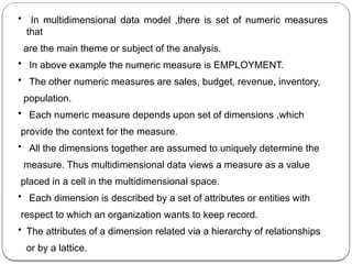
• In multidimensional data model ,there is set of numeric measures
that
are the main theme or subject of the analysis.
• In above example the numeric measure is EMPLOYMENT.
• The other numeric measures are sales, budget, revenue, inventory,
population.
• Each numeric measure depends upon set of dimensions ,which
provide the context for the measure.
• All the dimensions together are assumed to uniquely determine the
measure. Thus multidimensional data views a measure as a value
placed in a cell in the multidimensional space.
• Each dimension is described by a set of attributes or entities with
respect to which an organization wants to keep record.
• The attributes of a dimension related via a hierarchy of relationships
or by a lattice.

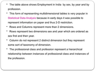
• The table above shows Employment in India by sex, by year and by
profession.
• This form of representing multidimensional tables is very popular in
Statistical Data Analysis because in early days it was possible to
represent information on paper and thus 2-D restriction.
• Rows and Columns represent more than 2 dimensions.
• Rows represent two dimensions sex and year which are ordered as
sex first and then year.
• Column do not represent 2 distinct dimension but they represent
some sort of taxonomy of dimension.
• The professional class and profession represent a hierarchical
relationship between instances of professional class and instances of
the profession.

Data Cube
An n-dimensional data cube C[A1,A2…..An ] is a database with n
dimensions as A1,A2 ……..An ,each of which represent a theme
and contains |Ai| number of distinct elements in the dimension Ai.
Each distinct element of Ai corresponds to a data row of C.A data
cell in the cube C[a1,a2,……an] stores the numeric measures of the
data for Ai=ai Vi Thus a data cell corresponds to an instantiation of
all dimensions.
C [sex, profession, year] is the data cube and data cell [male, civil
engineer, year] stores 2780 as its associated measure.
As |sex|=2,|profession|=6 and |year|=5 we have Three dimensions
with 2 ,6 and 5 rows respectively.

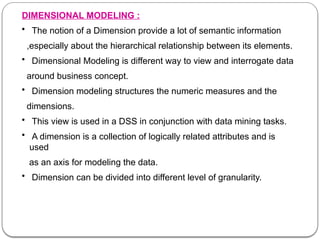
DIMENSIONAL MODELING :
• The notion of a Dimension provide a lot of semantic information
,especially about the hierarchical relationship between its elements.
• Dimensional Modeling is different way to view and interrogate data
around business concept.
• Dimension modeling structures the numeric measures and the
dimensions.
• This view is used in a DSS in conjunction with data mining tasks.
• A dimension is a collection of logically related attributes and is
used
as an axis for modeling the data.
• Dimension can be divided into different level of granularity.

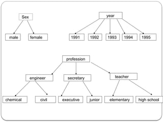
Sex
male female
year
1991 1992 1993 1994 1995
profession
engineer secretary teacher
chemical civil executive junior elementary high school

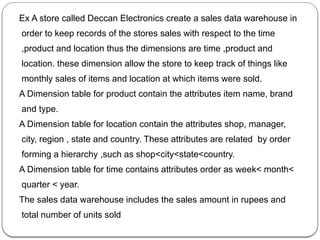
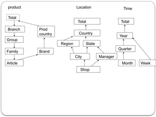
Ex A store called Deccan Electronics create a sales data warehouse in
order to keep records of the stores sales with respect to the time
,product and location thus the dimensions are time ,product and
location. these dimension allow the store to keep track of things like
monthly sales of items and location at which items were sold.
A Dimension table for product contain the attributes item name, brand
and type.
A Dimension table for location contain the attributes shop, manager,
city, region , state and country. These attributes are related by order
forming a hierarchy ,such as shop<city<state<country.
A Dimension table for time contains attributes order as week< month<
quarter < year.
The sales data warehouse includes the sales amount in rupees and
total number of units sold

Total
Branch
Group
Location
Family
Article
Brand
Prod
country
product
Total
Region State
Country
Year
City
Shop
Manager
Month Week
Total
Quarter
Time

Lattice of Cuboids :
Multidimensional data can be viewed as lattice of cuboids. The
C[A1,A2,…….An] at the finest level of granularity is called base
cuboid and it consist of all the data cells. The (n-1)-D cubes are
obtained by grouping the cells and computing the combined
numeric measure of a given dimension, Finally the coarsest
level
consists of one cell with numeric measures of all n dimensions
This is called an apex cuboid. In lattice of cuboids, all other
cuboids lie between the base cuboid and apex cuboid.
In above example the dimension hierarchy considered for the
data cube are time: (month<quarter<year);
location : (city<province<country) and product.

Base cuboid of lattice corresponds to C[ month ,city ,product] .
Apex cuboid of lattice corresponds to C[ year, country ,product]
Other intermediate cuboids in the lattice are
C[ quarter ,province ,product]
C[ quarter, country, product]
C[ month ,province ,product]
C[ month, country ,product]
C[ year ,city ,product]
C[ year ,province ,product]

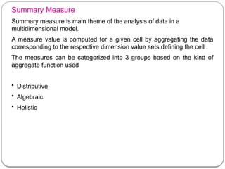
Summary Measure
Summary measure is main theme of the analysis of data in a
multidimensional model.
A measure value is computed for a given cell by aggregating the data
corresponding to the respective dimension value sets defining the cell .
The measures can be categorized into 3 groups based on the kind of
aggregate function used
• Distributive
• Algebraic
• Holistic

Distributive: A numeric measure is distributive if it can be
computed in a distributed manner.
Suppose the data is partitioned into a few subset. the measure can
be simply the aggregation of the measures of all partitions ex
count, sum, min, max etc.
Algebraic : An aggregate function is algebraic if it can be computed
by an algebraic function with some set of arguments, each of
which may be obtained by a distributive measure ex average
obtained by sum/count.
Holistic : An aggregate function is holistic if there is no constant
bound on the storage size needed to describe a sub aggregate.
That is ,there does not exist an algebraic function that can be used
to compute this function. Ex median, mode, most frequent

ONLINE ANALYTICAL PROCESSING (OLAP) :
• OLAP systems are targeted to provide more complex query results than
traditional OLTP or database systems.
• OLAP applications involve analysis of actual data through complex
query.
• It is an extension of some of the basic aggregation functions available
in SQL.
• OLAP tool may also be used in DSS system.
• OLAP operations are performed on data warehouse.
• Primary goal of OLAP is to support DSS .The multidimensional view of
the data is fundamental to OLAP operations.

OLAP tools classified as
 MOLAP (Multidimensional OLAP)
 ROLAP (Relational OLAP).
MOLAP (Multidimensional OLAP)
• Data are modeled, viewed and physically stored in a multidimensional
database(MDD).
• MOLAP tools are implemented by specialized DBMS and software
system capable of supporting the multidimensional data directly.
• Data are stored as n-dimensional array so the cube view is stored
directly.
• As MOLAP has extremely high storage requirements, indices are used
to speed up processing.

ROLAP (Relational OLAP)
• With ROLAP(relational OLAP) Data are stored in a relational database
and a ROLAP server (middleware) creates , the multidimensional view
for the user.
• ROLAP Tools tend to be less complex but also less efficient.
• MDD system may presummarize along all dimensions.
HOLAP (Hybrid OLAP)
• HOLAP combines the best features of ROLAP and MOLAP.
• Queries are stated in multidimensional terms.
• Data that are not updated frequently will be stored as MDD whereas
data that are updated frequently will be stored as RDB.

OLAP Operations supported by OLAP tools
A simple query may look at a single cell within the cube.
Slice : Look at a sub cube to get more specific information .This is
performed by selecting on one dimension, this is looking at a portion of
the cube.
Dice : Look at a sub cube by selecting on two or more dimensions .This
can be performed by a slice on one dimension and then rotating the
cube to select on a second dimension.
Roll Up (dimension reduction ,aggregation): Roll up allows the user to
ask
questions that move up an aggregation hierarchy.
Drill Down : These function allow a user to get more detailed fact
information by navigating lower in the aggregation hierarchy.
Visualization : Visualization allows the OLAP users to actually see results
of an operation.

WEB SEARCH ENGINE :
Web search engines are used to access the data and viewed as
query systems like IR system.
Like IR queries ,search engine queries can be stated as keyword,
Boolean and so on.
Difference is primarily in the data being searched ,pages with
heterogeneous data and extensive hyperlink and architecture
involved.
Conventional Search engines suffer from several problems.
• Abundance
• Limited Coverage
• Limited Query
• Limited Customization

Abundance : Although there is a lot of data on the web, an individual
query will retrieve only a small subset of it.
Limited Coverage : Search engine creates indices that are updated
Periodically . when a query is requested only index is directly accessed.
Limited Query : Most search engine provide access based on simple
keyword based searching. More advanced search engine retrieve or
order pages based on other properties such as popularity of pages.
Limited Customization :Query results are determined only by query itself
as with traditional IR systems, the desired results are dependent on the
background and knowledge of the user as well. More advanced search
engines add the ability to do customization using user profiles or
historical information.

Hypothesis Testing :
• Hypothesis testing attempts to find a model which explains observed
data by first creating Hypothesis and Testing Hypothesis against the
data.
• In data mining approach, first model is created from actual data
without guessing what it is first. Actual data itself derive the model
creation Hypothesis is verified by examining a simple data. If
Hypothesis holds for sample ,it is assumed to hold for population in
general.
• Given a population initial hypothesis to be tested H0 hypothesis is
called null hypothesis. Rejection of null hypothesis causes another
hypothesis H1 called Alternative Hypothesis to be made.
• One technique to perform Hypothesis Testing is based on the use of
Chi-squared Statistic.
• Actually there is a set of procedures referred to as chi squared.

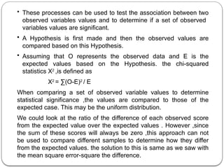
• These processes can be used to test the association between two
observed variables values and to determine if a set of observed
variables values are significant.
• A Hypothesis is first made and then the observed values are
compared based on this Hypothesis.
• Assuming that O represents the observed data and E is the
expected values based on the Hypothesis. the chi-squared
statistics X2
,is defined as
X2
= ∑(O-E)2
/ E
When comparing a set of observed variable values to determine
statistical significance ,the values are compared to those of the
expected case. This may be the uniform distribution.
We could look at the ratio of the difference of each observed score
from the expected value over the expected values . However ,since
the sum of these scores will always be zero ,this approach can not
be used to compare different samples to determine how they differ
from the expected values. the solution to this is same as we saw with
the mean square error-square the difference.

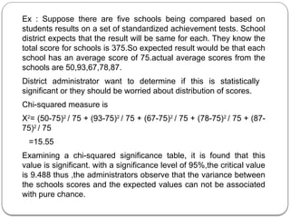
Ex : Suppose there are five schools being compared based on
students results on a set of standardized achievement tests. School
district expects that the result will be same for each. They know the
total score for schools is 375.So expected result would be that each
school has an average score of 75.actual average scores from the
schools are 50,93,67,78,87.
District administrator want to determine if this is statistically
significant or they should be worried about distribution of scores.
Chi-squared measure is
X2
= (50-75)2
/ 75 + (93-75)2
/ 75 + (67-75)2
/ 75 + (78-75)2
/ 75 + (87-
75)2
/ 75
=15.55
Examining a chi-squared significance table, it is found that this
value is significant. with a significance level of 95%,the critical value
is 9.488 thus ,the administrators observe that the variance between
the schools scores and the expected values can not be associated
with pure chance.

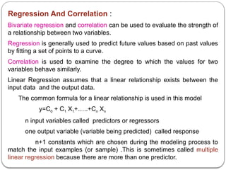
Regression And Correlation :
Bivariate regression and correlation can be used to evaluate the strength of
a relationship between two variables.
Regression is generally used to predict future values based on past values
by fitting a set of points to a curve.
Correlation is used to examine the degree to which the values for two
variables behave similarly.
Linear Regression assumes that a linear relationship exists between the
input data and the output data.
The common formula for a linear relationship is used in this model
y=C0 + C1 X1+…..+Cn Xn
n input variables called predictors or regressors
one output variable (variable being predicted) called response
n+1 constants which are chosen during the modeling process to
match the input examples (or sample) .This is sometimes called multiple
linear regression because there are more than one predictor.

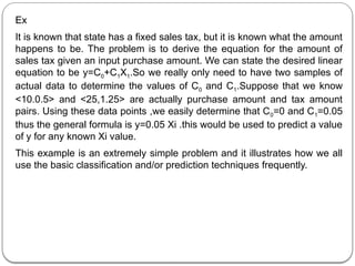
Ex
It is known that state has a fixed sales tax, but it is known what the amount
happens to be. The problem is to derive the equation for the amount of
sales tax given an input purchase amount. We can state the desired linear
equation to be y=C0+C1X1.So we really only need to have two samples of
actual data to determine the values of C0 and C1.Suppose that we know
<10.0.5> and <25,1.25> are actually purchase amount and tax amount
pairs. Using these data points ,we easily determine that C0=0 and C1=0.05
thus the general formula is y=0.05 Xi .this would be used to predict a value
of y for any known Xi value.
This example is an extremely simple problem and it illustrates how we all
use the basic classification and/or prediction techniques frequently.

1
2
3
4
5
6
7
8
9
10
11
12
1 2 3 4 5 6 7 8 9
10

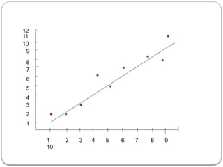
The fig above illustrate the more general use of Linear regression with
one input value. Here we have a sample of data we wish to model
using a linear model. The line generated by the linear regression
technique is shown in fig .The actual point do not fit the linear model
exactly. Thus ,this model is an estimate of what the actual input-output
relationship is. We can use the generated linear model to predict an
output value given an input value.
Two different data variables X and Y. may behave similarly. Correlation
is the problem of determining how much alike the two variables
actually are.
One standard formula to measure linear correlation is correlation
coefficient r.
Given two variables X and Y the correlation coefficient is a real value r
Є[-1,1]
Positive number indicates positive correlation
Negative number indicates negative correlation means that one
variable increases while other decreases In value.
Closer the value of r to 0 the smaller the correlation.

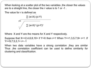
When looking at a scatter plot of the two variables ,the closer the values
are to a straight line, the closer the r value is to 1 or -1 .
The value for r is defined as
∑ (xi-X) (yi-Y)
r=
∑ (xi-X)2
(yi-Y)2
Where X and Y are the means for X and Y respectively.
Suppose that X=<2,4,6,8,10> if Y=X then r=1 When Y=<1,3,5,7,9> r=1 .If
Y=<9,7,5,3,1> r= -1
When two data variables have a strong correlation ,they are similar
Thus ,the correlation coefficient can be used to define similarity for
clustering and classification.

Similarity Measures:
In Internet searching ,the set of all web pages represent whole
database and these are divided into two classes those that answer
query and those that do not answer query.
Those that answer your query should be much like each other than
those that do not answer your query.
Similarity is defined by query you state ,usually based on keyword list
thus retrieved pages are similar because they all contain similar
keywords.
Idea of Similarity measures can be abstracted and applied to more
general classification problem. difficulty lies in how similarity measure
are defined and applied to items in the database. most of the similarity
measure assume numeric values they may be difficult to use for more
general data types. A mapping from more general attribute domain to a
subset of integers may be used.

Definition : Similarity between two tuples ti and tj Sim(ti,tj) in a database is
a mapping from D*D to range[0,1] thus Sim(ti,tj) Є [0,1].
Desirable characteristics of Good Similarity Measure
1. ν ti Є D Sim(ti,tj)=1
2. ν ti tj Є D Sim(ti,tj)=0 if ti and tj are not alike at all.
3. ν ti tj,tk Є D Sim(ti,tj) < Sim(tj,tk) if ti is more like tk then it is more like tj.
Defining Similarity measure is difficult part often concept of alikeness is
itself not well defined .When idea of Similarity measures is used in
classification where classes are predefined this problem is somewhat
easier than when it is used for clustering where classes are not known
in advance.

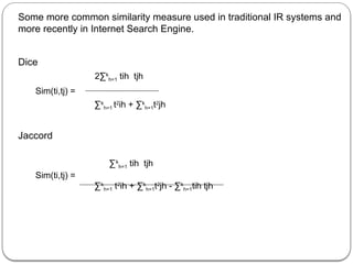
Some more common similarity measure used in traditional IR systems and
more recently in Internet Search Engine.
Dice
2∑k
h=1 tih tjh
Sim(ti,tj) =
∑k
h=1 t2
ih + ∑k
h=1t2
jh
Jaccord
∑k
h=1 tih tjh
Sim(ti,tj) =
∑k
h=1 t2
ih + ∑k
h=1t2
jh - ∑k
h=1tih tjh

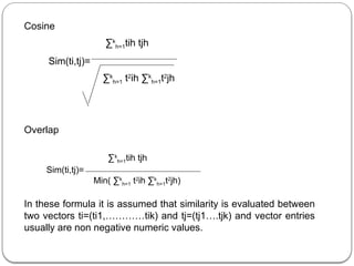
Cosine
∑k
h=1tih tjh
Sim(ti,tj)=
∑k
h=1 t2
ih ∑k
h=1t2
jh
Overlap
∑k
h=1tih tjh
Sim(ti,tj)=
Min( ∑k
h=1 t2
ih ∑k
h=1t2
jh)
In these formula it is assumed that similarity is evaluated between
two vectors ti=(ti1,…………tik) and tj=(tj1….tjk) and vector entries
usually are non negative numeric values.

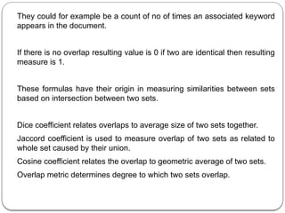
They could for example be a count of no of times an associated keyword
appears in the document.
If there is no overlap resulting value is 0 if two are identical then resulting
measure is 1.
These formulas have their origin in measuring similarities between sets
based on intersection between two sets.
Dice coefficient relates overlaps to average size of two sets together.
Jaccord coefficient is used to measure overlap of two sets as related to
whole set caused by their union.
Cosine coefficient relates the overlap to geometric average of two sets.
Overlap metric determines degree to which two sets overlap.

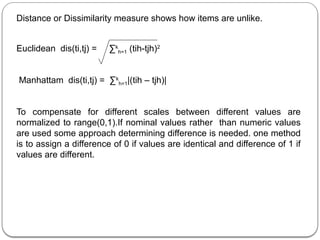
Distance or Dissimilarity measure shows how items are unlike.
Euclidean dis(ti,tj) = ∑k
h=1 (tih-tjh)2
Manhattam dis(ti,tj) = ∑k
h=1|(tih – tjh)|
To compensate for different scales between different values are
normalized to range(0,1).If nominal values rather than numeric values
are used some approach determining difference is needed. one method
is to assign a difference of 0 if values are identical and difference of 1 if
values are different.

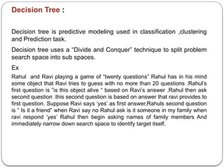
Decision Tree :
Decision tree is predictive modeling used in classification ,clustering
and Prediction task.
Decision tree uses a “Divide and Conquer” technique to split problem
search space into sub spaces.
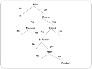
Ex
Rahul and Ravi playing a game of “twenty questions” Rahul has in his mind
some object that Ravi tries to guess with no more than 20 questions .Rahul’s
first question is ”is this object alive “ based on Ravi’s answer .Rahul then ask
second question .this second question is based on answer that ravi provides to
first question. Suppose Ravi says ‘yes’ as first answer,Rahuls second question
is “ Is it a friend” when Ravi say no Rahul ask is it someone in my family when
ravi respond ‘yes’ Rahul then begin asking names of family members And
immediately narrow down search space to identify target itself.

Alive
No
yes
No
Person
yes
No
Mammal Friend
No yes
yes
In Family
No
No
yes
Mom
No yes
Finished

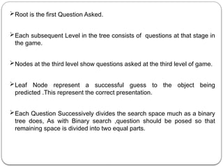
Root is the first Question Asked.
Each subsequent Level in the tree consists of questions at that stage in
the game.
Nodes at the third level show questions asked at the third level of game.
Leaf Node represent a successful guess to the object being
predicted .This represent the correct presentation.
Each Question Successively divides the search space much as a binary
tree does, As with Binary search ,question should be posed so that
remaining space is divided into two equal parts.

Definition :
Decision tree is a tree where root and each internal node is labeled with a
question. Arc emitting from each node represent possible answer to
associated question and leaf node represent a prediction of a solution to
the problem under consideration.
A decision tree model is a computational model consisting of three parts.
A Decision tree defined above.
An Algorithm to create tree.
An Algorithm that applies to data and solves the problem under
consideration.
Building of a tree may be accomplished via an algorithm that examines
data from a training sample or could be created by domain expert.

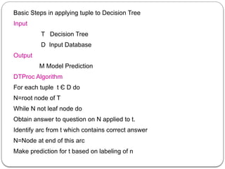
Basic Steps in applying tuple to Decision Tree
Input
T Decision Tree
D Input Database
Output
M Model Prediction
DTProc Algorithm
For each tuple t Є D do
N=root node of T
While N not leaf node do
Obtain answer to question on N applied to t.
Identify arc from t which contains correct answer
N=Node at end of this arc
Make prediction for t based on labeling of n

Complexity of algorithm is straight forward to analyze
For each tuple in the database ,we search tree from root down to a
particular leaf. At each level ,maximum no of comparisons to make
depends upon branching factor at that level. so complexity depends on
the product of no of levels and maximum branching factor.
Ex Suppose student in a particular university are classified as short, tall.
medium based on their height assume database schema is {name,
address, gender, height, age, year, major} to construct a decision tree we
must identify attribute that are important to classification problem at hand
and attribute chosen is height, gender and age.
1.A female who is 1.95 m in height is considered tall while a male of the
same height may not be considered tall
2.A child of 10 years of age may be tall if he or she is only 1.5 m.
Since this is set of university students we expect more of them to be over
17 years of age so we decide to filter out database under this age and
perform classification separately.

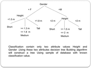
Gender
= F =M
Height
>2 m
>1.8 m
Short Tall
>= 1.5 m
<= 2 m
Medium
Height
>2 m
<1.5 m
Short
Tall
>= 1.3 m
<= 1.8 m
Medium
Classification contain only two attribute values Height and
Gender .Using these two attributes decision tree Building algorithm
will construct a tree Using sample of database with known
classification value.

Genetic Algorithm :
Genetic Algorithm are evolutionary computing method and are
optimization type algorithm.
Given a population of potential problem solutions (individual) Evolutionary
computing expands this population with new and potentially better
solution.
Basis for evolutionary computing algorithm is biological evolution ,where
over time evolution produces best or fittest individuals. chromosomes
which are DNA strings provide abstract model for living organisms.
Subsections of chromosomes which are called Genes are used to define
different traits of individual. During reproduction genes from parents
combined to produce Genes for child.
In data mining, Genetic algorithm used for clustering ,classification and
association rules.

This technique finds “fittest models” from a set of models to represent
data .In this approach a starting model is assumed and through many
iterations models are combined to create new models .The best of
these is defined by a fitness function are then input to next iteration.
Algorithm differ in how model is represented ,how different individual in
the model are combined and how fitness function is used.
Using Genetic algorithm to solve a problem. the most difficult part is
how to model problem as set of individuals .In real world individuals
may be identified .complete encoding of DNA structure. An individual is
viewed as an array or tuple of values, Based on recombination
algorithm the values are usually numeric or may be binary string.
these individuals are like DNA encoding that the structure for each
individual represent an encoding of major features needed to model
the problem.
Each individual in the population is represented as a string of
characters from given alphabet.

Definition:
Given an alphabet A an individual or chromosome is a string I=I1,I2,
……..In where Ij Є A .Each character in the string Ij is called a Gene
values that each character can have are called alleles. A population is set
of individuals.
In Genetic algorithm reproduction is defined by algorithm that indicate how
to combine given set of individuals to produce new ones called Crossover
algorithm.
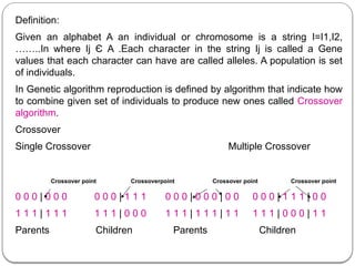
Crossover
Single Crossover Multiple Crossover
Crossover point Crossoverpoint Crossover point Crossover point
0 0 0 | 0 0 0 0 0 0 | 1 1 1 0 0 0 | 0 0 0 | 0 0 0 0 0 | 1 1 1 | 0 0
1 1 1 | 1 1 1 1 1 1 | 0 0 0 1 1 1 | 1 1 1 | 1 1 1 1 1 | 0 0 0 | 1 1
Parents Children Parents Children

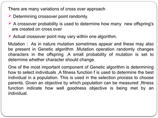
There are many variations of cross over approach
 Determining crossover point randomly.
 A crossover probability is used to determine how many new offspring's
are created on cross over
 Actual crossover point may vary within one algorithm.
Mutation : As in nature mutation sometimes appear and these may also
be present in Genetic algorithm .Mutation operation randomly changes
characters in the offspring .A small probability of mutation is set to
determine whether character should change.
One of the most important component of Genetic algorithm is determining
how to select individuals ,A fitness function f is used to determine the best
individual in a population. This is used in the selection process to choose
parents. Given an objective by which population can be measured ,fitness
function indicate how well goodness objective is being met by an
individual.

Definition :
Genetic Algorithm is computational model consisting of five parts
1.Starting set of individual P.
2. Crossover technique.
3. Mutation algorithm.
4. Fitness Function.
5. Algorithm that applies the crossover and mutation technique to P
iteratively using the fitness function to determine best individual in P to
keep. The algorithm replaces a predefined no of individuals from
population with each iteration and terminates when some threshold is
met.

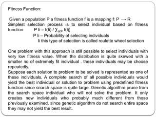
Fitness Function:
Given a population P a fitness function f is a mapping f: P R
Simplest selection process is to select individual based on fitness
function P Ii = f(Ii) / ∑IjЄP f(Ij)
P Ii – Probability of selecting individuals
Ii this type of selection is called roulette wheel selection
One problem with this approach is still possible to select individuals with
very low fitness value. When the distribution is quite skewed with a
smaller no of extremely fit individual . these individuals may be choose
repeatedly.
Suppose each solution to problem to be solved is represented as one of
these individuals. A complete search of all possible individuals would
yield the best individual or solution to problem using predefined fitness
function since search space is quite large. Genetic algorithm prune from
the search space individual who will not solve the problem. It only
creates new individuals who probably much different from those
previously examined. since genetic algorithm do not search entire space
they may not yield the best result.

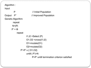
Algorithm :
Input
P // Initial Population
Output P” // Improved Population
Genetic Algorithm
repeat
N=|P|
P’ = Φ
repeat
I1,I2 =Select (P)
O1,O2 =cross(I1,I2)
O1=mutate(O1)
O2=mutate(O2)
P’=P’ υ { O1,O2}
untill | P’|=N
P=P’ untill termination criterion satisfied

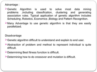
Advantage :
Genetic Algorithm is used to solve most data mining
problems ,including classification, clustering and generating
association rules. Typical application of genetic algorithm includes
Scheduling ,Robotics, Economics ,Biology and Pattern Recognition.
Many Advantage to use genetic algorithm is that they are easily
parallelized.
Disadvantage
Genetic algorithm difficult to understand and explain to end user.
Abstraction of problem and method to represent individual is quite
difficult.
Determining Best fitness function is difficult.
Determining how to do crossover and mutation is difficult.

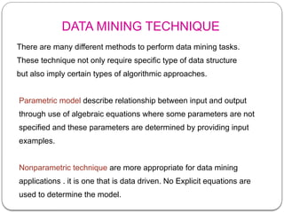
DATA MINING TECHNIQUE
There are many different methods to perform data mining tasks.
These technique not only require specific type of data structure
but also imply certain types of algorithmic approaches.
Parametric model describe relationship between input and output
through use of algebraic equations where some parameters are not
specified and these parameters are determined by providing input
examples.
Nonparametric technique are more appropriate for data mining
applications . it is one that is data driven. No Explicit equations are
used to determine the model.

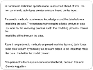
In Parametric technique specific model is assumed ahead of time, the
non parametric techniques creates a model based on the input.
Parametric methods require more knowledge about the data before a
modeling process. The non parametric require a large amount of data
as input to the modeling process itself. the modeling process creates
the
model by sifting through the data.
Recent nonparametric methods employed machine learning techniques
to be able to learn dynamically as data are added to the input thus more
the data , the better the model created.
Non parametric techniques include neural network, decision tree and
Genetic Algorithm

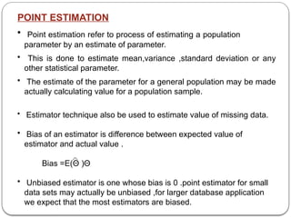
POINT ESTIMATION
• Point estimation refer to process of estimating a population
parameter by an estimate of parameter.
• This is done to estimate mean,variance ,standard deviation or any
other statistical parameter.
• The estimate of the parameter for a general population may be made
actually calculating value for a population sample.
• Estimator technique also be used to estimate value of missing data.
• Bias of an estimator is difference between expected value of
estimator and actual value .
Bias =E(Θ )
Θ
• Unbiased estimator is one whose bias is 0 .point estimator for small
data sets may actually be unbiased ,for larger database application
we expect that the most estimators are biased.

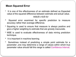
• It is one of the effectiveness of an estimate defined as Expected
value of the squared difference between estimate and actual value.
MSE(Θ )=E(Θ
Θ)2
• Squared error examined for specific prediction to measure
accuracy rather than average difference.
• Squaring is used to ensure that measure is always positive and
give a higher weighting to estimate that are grossly inaccurate.
• MSE is used to evaluate effectiveness of data mining prediction
technique.
• It is important in machine learning.
• Sometimes instead of predicting a simple point estimate for a
parameter ,one may determine a range of values within which true
parameter value should fall this range is called Confidence Interval.
Mean Squared Error

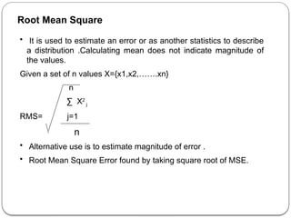
Root Mean Square
• It is used to estimate an error or as another statistics to describe
a distribution .Calculating mean does not indicate magnitude of
the values.
Given a set of n values X={x1,x2,…….xn}
n
∑ X2
j
RMS= j=1
n
• Alternative use is to estimate magnitude of error .
• Root Mean Square Error found by taking square root of MSE.

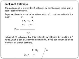
Jackkniff Estimate
The estimate of a parameter Θ obtained by omitting one value from a
set of observed values.
Suppose there is a set of n values x={x1,x2,…xn} an estimate for
mean i-1 n
∑ Xj + ∑ X j
j=1 j=i+1
µ( I ) =
n-1
Subscript (i) indicates that this estimate is obtained by omitting i th
value.Given a set of Jackknife estimate Θ(i) these can in turn be used
to obtain an overall estimate.
n
∑ Θ(j) n
Θ(.) = j=1

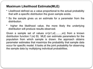
Maximum Likelihood Estimate(MLE)
• Likelihood defined as a value proportional to the actual probability
that with a specific distribution the given sample exists.
• So the sample gives us an estimate for a parameter from the
distribution.
• higher the likelihood value, the more likely the underlying
distribution will produce results observed.
Given a sample set of values x={x1,x2,……,xn} from a known
distribution function f (xi| Θ) MLE can estimate parameters for the
population from which sample is drawn. the approach obtains
parameter estimates that maximize the probability that sample data
occur for specific model. It looks at the joint probability for observing
the sample data by multiplying individual probabilities.

Likelihood function L is defined as
n
L(Θ | X1,X2,........Xn) = Π f (Xi | Θ)
i=1
The value of Θ that maximizes L is the estimate chosen .This can be
found by taking the derivative with respect to Θ.

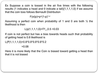
Ex Suppose a coin is tossed in the air five times with the following
results (1 indicates a head and 0 indicate a tail){1,1,1,1,0} if we assume
that the coin toss follows Bernaulli Distribution
F(xi|p)=pxi
(1-p)1-xi
Assuming a perfect coin when probability of 1 and 0 are both ½ the
likelihood is then
L(p|1,1,1,1,0)=Π5
i=10.5 =0.03
If coin is not perfect but has a bias towards heads such that probability
of getting head is 0.8 likelihood is
L(P|1,1,1,1,0)=0.8*0.8*0.8*0.8*0.2
=0.08
Here it is more likely that the Coin is biased toward getting a head than
that it is not biased

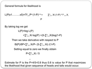
General formula for likelihood is
L(P|x1………x5)=Π5
i=1Pxi
(1-P)1-xi
= ∑5
i=1 Xi (1-P) 5-∑5
i=1 Xi
P
By taking log we get
L(P)=log L(P)
=∑5
i=1 Xi log(P) +(5-∑5
i=1Xi)log(1-P)
Then we take derivative with respect to P
δl(P)/δP=∑5
i=1 Xi/P- (5-∑5
i=1 Xi) /(1-P)
Setting equal to zero we finally obtain
P=∑5
i=1Xi / 5
Estimate for P is the P=4/5=0.8 thus 0.8 is value for P that maximizes
the likelihood that given sequence of heads and tails would occur.

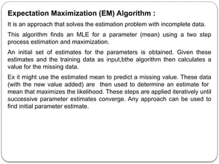
Expectation Maximization (EM) Algorithm :
It is an approach that solves the estimation problem with incomplete data.
This algorithm finds an MLE for a parameter (mean) using a two step
process estimation and maximization.
An initial set of estimates for the parameters is obtained. Given these
estimates and the training data as input,bthe algorithm then calculates a
value for the missing data.
Ex it might use the estimated mean to predict a missing value. These data
(with the new value added) are then used to determine an estimate for
mean that maximizes the likelihood. These steps are applied iteratively until
successive parameter estimates converge. Any approach can be used to
find initial parameter estimate.

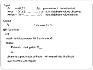
Input
Θ = {θ1,θ2,…………,θp) parameters to be estimated
Xobs = {x1,x2,……………,xk) input database values observed
Xmiss = {Xk+1…………….Xn) input database value missing
Output
Θ Estimates for Θ
EM Algorithm
i=0
obtain initial parameter MLE estimate, Θi
repeat
Estimate missing data Xi
miss
i++
obtain next parameter estimate ,θ i
to maximize likelihood;
untill estimate converges;

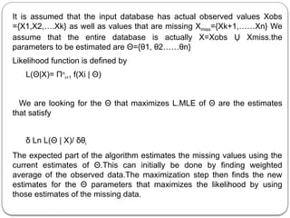
It is assumed that the input database has actual observed values Xobs
={X1,X2,….Xk} as well as values that are missing Xmiss={Xk+1,……Xn} We
assume that the entire database is actually X=Xobs Ụ Xmiss.the
parameters to be estimated are Θ={θ1, θ2……θn}
Likelihood function is defined by
L(Θ|X)= Πn
i=1 f(Xi | Θ)
We are looking for the Θ that maximizes L.MLE of Θ are the estimates
that satisfy
δ Ln L(Θ | X)/ δθi
The expected part of the algorithm estimates the missing values using the
current estimates of Θ.This can initially be done by finding weighted
average of the observed data.The maximization step then finds the new
estimates for the Θ parameters that maximizes the likelihood by using
those estimates of the missing data.

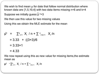
We wish to find mean µ for date that follow normal distribution where
known data are {1,5,10,4} with two data items missing n=6 and k=4
Suppose we initially guess µ 0
=3
We then use this value for two missing values
Using this we obtain the MLE estimate for the mean
µ1
= ∑k
i=1 Xi / n + ∑ n
i=k+1 Xi /n
= 3.33 + ((3+3)/6
= 3.33+1
= 4.33
We now repeat using this as new value for missing items,the estimate
mean as
µ2 =
∑k
i=1 Xi / n + ∑ n
i=k+1 Xi /n

=3.33+(4.33+4.33)/6=4.77
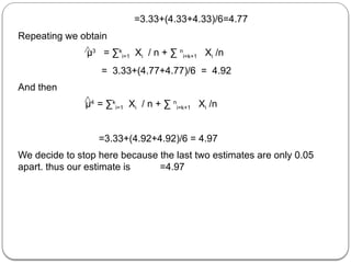
Repeating we obtain
µ3
= ∑k
i=1 Xi / n + ∑ n
i=k+1 Xi /n
= 3.33+(4.77+4.77)/6 = 4.92
And then
µ4
= ∑k
i=1 Xi / n + ∑ n
i=k+1 Xi /n
=3.33+(4.92+4.92)/6 = 4.97
We decide to stop here because the last two estimates are only 0.05
apart. thus our estimate is =4.97

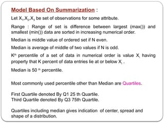
Model Based On Summarization :
Let X1,X2,X3 be set of observations for some attribute.
Range : Range of set is difference between largest (max()) and
smallest (min()) data are sorted in increasing numerical order.
Median is middle value of ordered set if N even.
Median is average of middle of two values if N is odd.
Kth
percentile of a set of data in numerical order is value Xi having
property that K percent of data entries lie at or below Xi .
Median is 50 th
percentile.
Most commonly used percentile other than Median are Quartiles.
First Quartile denoted By Q1 25 th Quartile.
Third Quartile denoted By Q3 75th Quartile.
Quartiles including median gives indication of center, spread and
shape of a distribution.

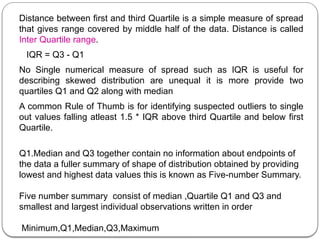
Distance between first and third Quartile is a simple measure of spread
that gives range covered by middle half of the data. Distance is called
Inter Quartile range.
IQR = Q3 - Q1
No Single numerical measure of spread such as IQR is useful for
describing skewed distribution are unequal it is more provide two
quartiles Q1 and Q2 along with median
A common Rule of Thumb is for identifying suspected outliers to single
out values falling atleast 1.5 * IQR above third Quartile and below first
Quartile.
Q1.Median and Q3 together contain no information about endpoints of
the data a fuller summary of shape of distribution obtained by providing
lowest and highest data values this is known as Five-number Summary.
Five number summary consist of median ,Quartile Q1 and Q3 and
smallest and largest individual observations written in order
Minimum,Q1,Median,Q3,Maximum

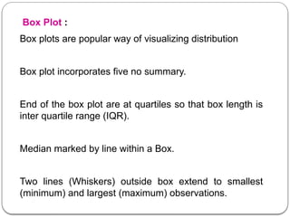
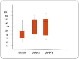
Box Plot :
Box plots are popular way of visualizing distribution
Box plot incorporates five no summary.
End of the box plot are at quartiles so that box length is
inter quartile range (IQR).
Median marked by line within a Box.
Two lines (Whiskers) outside box extend to smallest
(minimum) and largest (maximum) observations.

20
40
60
80
100
120
140
160
180
200
Branch1 Branch 2 Branch 3

When dealing with moderate number of observations it is worthwhile to
plot potential outlier individually. To do this in Boxplot whiskers are
extended to extreme low and high observations. If these values are
less than 1.5 IQR beyond quartiles otherwise whiskers terminate at
most extreme observations occurring within 1.5*IQR of Quartiles
Efficient computation of Box plots or even approximate Boxplot (Based
on approximate of five number summary) remains a challenging issue
for mining large data set.

Scatter Diagram
It is visual technique to display data.
This is a graph on two dimensional axis of points representing
relationship between x and y values.
By plotting actually observable (x,y) points as seen in sample visual
image of some derivable functional relationship between x and y values
in total population may be seen.
Even though points do not lie on a precisely linear line they do hint this
may be a good predictor of relationship between x and y.

Bayes Theorem :
• With statistical inference ,information about data distribution inferred
by examining data that follows that distribution.
• Given a set of data X={x1,x2,……..xn} a data mining problem is to
understand properties of the distribution from which set comes.
• Bayes Rule Is a technique to estimate likelihood of a property given
set of data as evidence or input .Suppose that either hypothesis h1 or
hypothesis h2 must occur but not both. Also suppose that xi is an
observable event.

Bayes rule or Bayes Theorem is:
P(h1/Xi)=P(Xi|h1)P(h1) / ( P(Xi|h1)P(h1)+P(Xi|h2)(P(h2))
P(h1/Xi) Posterior Probability.
P(h1) Prior Probability associated with Hypothesis h1
P(Xi) Is the probability of the occurances of data value Xi
P(Xi|h1) conditional Probability that given hypothesis tuple satisfies it.
Where there are m different Hypothesis
P(Xi)=∑m
j=1 P(Xi|hj)P(hj)
Thus we have
P(h1|Xi)=P(Xi|h1)P(h1)/P(Xi)

Thus Bayes Rule allows to assign probabilities of hypothesis given a data
value, P(hj|Xi)
Here we discuss tuples when in actuality each Xi may be an attribute value or
other data label. Each hi may be an attribute value or ,set of attribute values
or even a combination of attribute values.
Example
Suppose that a credit loan authorization problem can be associated with four
hypothesis H={h1,h2,h3,h4} where
h1=authorize purchase
h2=authorize after further identification
H3= do not authorize
H4 =do not authorize but contact police.

Training data
ID Income Credit Class Xi
1 4 Excellent h1 X4
2 3 Good h1 X7
3 2 Excellent h1 X2
4 3 Good h1 X7
5 4 Good H1 X8
6 2 Excellent h1 X2
7 3 Bad H2 X11
8 2 Bad H2 X10
9 3 Bad h3 X11
10 1 Bad h4 X9

P(h1)=60% P(h2)=20% P(h3)=10% P(h4)=10%
To make predictions a domain expert has determined that the attributes we
should be looking at our income and credit category
Assume that income categorized by ranges
[0,$10,000],[$10,000,$50,000],[$50,000,$100000],[$100000,∞] these
ranges are encoded in table as 1,2,3,4 resply.
Suppose credit is categorized as excellent, good or bad. By combining
these we have 12 values in data space D={x1,x2…x12} relationship
between xi values and attributes shown as

1 2 3 4
Excellent x1 x2 x3 x4
Good x5 x6 x7 x8
Bad x9 x10 x11 x12
xi group into which that tuple falls.
Given these we can then calculate
P(xi|hj) and P(xi)
There are six tuples fro training set that are in h1.
Distribution of these across xi
P(x2 | h1)=2/6
P(x4 | h1) =1/6
P(x7 | h1) =2/6

P(x8 | h1) = 1/6
P(X9 | h1) =1/6
P(X10 | h1 ) =1/6
P(x11 | h1 ) = 2/6
For all other values of I P(Xi | h1)=0
Suppose we need to predict the class for x4 thus we need to find
P(hj | x4) for each hj
We would classify x4 to class with largest value for h1
P(h1|x4)=(1/6 * 0.6)/((1/6)*0.6)=0.1/0.1=1 thus classify x4 to h1.

The above example illustrate some issues associated with sampling.
1.Training data has no entries for X1,X3,X5,X6 or X12 .This makes it
impossible to use this training sample to determine how to make
predictions for these combination of input data. If these combination
donot occur then there is no problem.
2.Another issue with this sampling is its Size. of course sample of this
size is too small. Size of course is not only a criterion.

DWDM_UNIT4.pptx ddddddddddddddddddddddddddddd

More Related Content

Similar to DWDM_UNIT4.pptx ddddddddddddddddddddddddddddd

Recently uploaded

DWDM_UNIT4.pptx ddddddddddddddddddddddddddddd