Downloaded 184 times
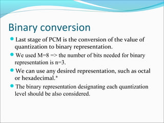
![Quantization
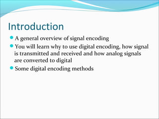
Confine the infinite set to finite set of values, defined
by letter M which is an exponential function
M = 2n
It can be easily derived from
the above table that this
quantizer has 8 levels (M=8).
The quantizer used here
is a linear quantizer.
Speech contain lower frequencies then higher
therefore we use more quantization levels then higher
X, the input voltage
[Volt]
Output voltage [Volt]
X >= 6 7
6 > X >= 4 5
4 > X >= 2 3
2 > X >= 0 1
0 > X >= -2 -1
-2 > X >= -4 -3
-4 > X >= -6 -5
-6 > X -7](https://image.slidesharecdn.com/1-pcmencoding-101102195735-phpapp01/85/1-PCM-Encoding-8-320.jpg)


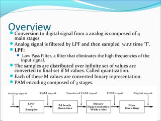
![Gray codes
Gray code can be very useful here.
In Gray code, every two neighboring words are different
in only one bit.
Thus a error caused due to additive noise will cause only
a minor shift to neighboring frequencies
Decreasing the impact of the
error occurred significantly.
Quantizer output voltage
[Volt]
PCM output [binary
representation]
7 110
5 111
3 101
1 100
-1 000
-3 001
-5 011
-7 010](https://image.slidesharecdn.com/1-pcmencoding-101102195735-phpapp01/85/1-PCM-Encoding-13-320.jpg)


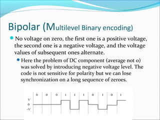


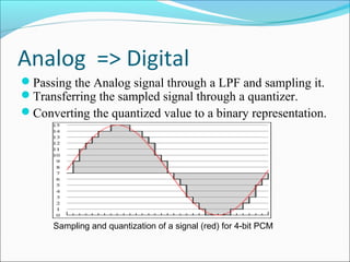
The document provides an overview of signal encoding, focusing on the conversion of analog signals to digital form through various stages like filtering, sampling, and quantization. It discusses different encoding methods, advantages of digital encoding, error correction, and the significance of modulation techniques. Key challenges such as quantization noise and inter-symbol interference, along with solutions like scrambling techniques, are also addressed.


![Chinua Achebe - Things Fall Apart [Edited Version]](https://cdn.slidesharecdn.com/ss_thumbnails/chinuaachebe-thingsfallapart2-130806172255-phpapp02-thumbnail.jpg?width=640&height=640&fit=bounds)


