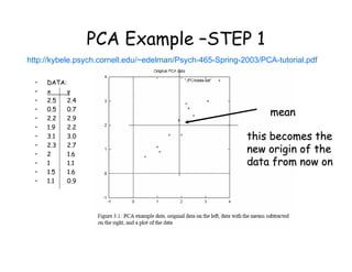
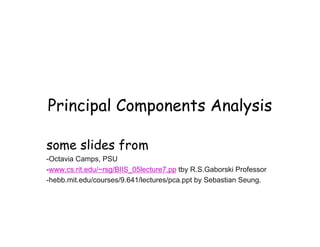
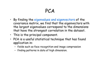
Principal Components Analysis (PCA) is a technique used to simplify complex datasets. It works by transforming the data to a new coordinate system where the greatest variance lies on the first axis (called the first principal component), second greatest variance on the second axis, and so on. This allows for dimensionality reduction by removing later principal components with less variance. PCA is commonly used for applications like face recognition, image compression, and finding patterns in high-dimensional data.

1. Principal Components Analysis
some slides from
-Octavia Camps, PSU
-www.cs.rit.edu/~rsg/BIIS_05lecture7.pp tby R.S.Gaborski Professor
-hebb.mit.edu/courses/9.641/lectures/pca.ppt by Sebastian Seung.

2. Covariance
• Variance and Covariance are a measure of the “spread” of a set
of points around their center of mass (mean)
• Variance – measure of the deviation from the mean for points in
one dimension e.g. heights
• Covariance as a measure of how much each of the dimensions
vary from the mean with respect to each other.
• Covariance is measured between 2 dimensions to see if there is
a relationship between the 2 dimensions e.g. number of hours
studied & marks obtained.
• The covariance between one dimension and itself is the variance

3. covariance (X,Y) = i=1 (Xi – X) (Yi – Y)
(n -1)
• So, if you had a 3-dimensional data set (x,y,z), then you could
measure the covariance between the x and y dimensions, the y
and z dimensions, and the x and z dimensions. Measuring the
covariance between x and x , or y and y , or z and z would give
you the variance of the x , y and z dimensions respectively.
Covariance
n
n

4. Covariance Matrix
• Representing Covariance between dimensions as a
matrix e.g. for 3 dimensions:
cov(x,x) cov(x,y) cov(x,z)
C = cov(y,x) cov(y,y) cov(y,z)
cov(z,x) cov(z,y) cov(z,z)
• Diagonal is the variances of x, y and z
• cov(x,y) = cov(y,x) hence matrix is symmetrical about
the diagonal
• N-dimensional data will result in NxN covariance
matrix
Variances

5. Covariance
• What is the interpretation of covariance
calculations?
e.g.: 2 dimensional data set
x: number of hours studied for a subject
y: marks obtained in that subject
covariance value is say: 104.53
what does this value mean?

6. Covariance examples
X
Y

7. Covariance
• Exact value is not as important as it’s sign.
• A positive value of covariance indicates both
dimensions increase or decrease together e.g. as the
number of hours studied increases, the marks in that
subject increase.
• A negative value indicates while one increases the
other decreases, or vice-versa e.g. active social life
at PSU vs performance in CS dept.
• If covariance is zero: the two dimensions are
independent of each other e.g. heights of students vs
the marks obtained in a subject

8. Covariance
• Why bother with calculating covariance
when we could just plot the 2 values to
see their relationship?
Covariance calculations are used to find
relationships between dimensions in high
dimensional data sets (usually greater
than 3) where visualization is difficult.

9. PCA
• principal components analysis (PCA) is a technique
that can be used to simplify a dataset
• It is a linear transformation that chooses a new
coordinate system for the data set such that
greatest variance by any projection of the data
set comes to lie on the first axis (then called the
first principal component),
the second greatest variance on the second axis,
and so on.
• PCA can be used for reducing dimensionality by
eliminating the later principal components.

10. PCA Toy Example
Consider the following 3D points
Consider the following 3D points
1
1
2
2
3
3
2
2
4
4
6
6
4
4
8
8
12
12
3
3
6
6
9
9
5
5
10
10
15
15
6
6
12
12
18
18
If each component is stored in a byte,
If each component is stored in a byte,
we need 18 = 3 x 6 bytes
we need 18 = 3 x 6 bytes

11. PCA Toy Example
Looking closer, we can see that all the points are related
Looking closer, we can see that all the points are related
geometrically: they are all the same point, scaled by a
geometrically: they are all the same point, scaled by a
factor:
factor:
1
1
2
2
3
3
4
4
8
8
12
12
3
3
6
6
9
9
5
5
10
10
15
15
6
6
12
12
18
18
= 1 *
= 1 *
1
1
2
2
3
3
= 4 *
= 4 *
1
1
2
2
3
3
= 3 *
= 3 *
1
1
2
2
3
3
= 5 *
= 5 *
1
1
2
2
3
3
= 6 *
= 6 *
2
2
4
4
6
6
= 2 *
= 2 *
1
1
2
2
3
3
1
1
2
2
3
3

12. PCA Toy Example
1
1
2
2
3
3
4
4
8
8
12
12
3
3
6
6
9
9
5
5
10
10
15
15
6
6
12
12
18
18
= 1 *
= 1 *
1
1
2
2
3
3
= 4 *
= 4 *
1
1
2
2
3
3
= 3 *
= 3 *
1
1
2
2
3
3
= 5 *
= 5 *
1
1
2
2
3
3
= 6 *
= 6 *
2
2
4
4
6
6
= 2 *
= 2 *
1
1
2
2
3
3
1
1
2
2
3
3
They can be stored using only 9 bytes (50% savings!):
They can be stored using only 9 bytes (50% savings!):
Store one point
Store one point (3 bytes)
(3 bytes) + the multiplying constants
+ the multiplying constants (6 bytes)
(6 bytes)

13. Geometrical Interpretation:
View each point in 3D space.
View each point in 3D space.
p1
p1
p2
p2
p3
p3
But in this example, all the points happen to belong to a
But in this example, all the points happen to belong to a
line: a 1D subspace of the original 3D space.
line: a 1D subspace of the original 3D space.

14. Geometrical Interpretation:
Consider a new coordinate system where one of the axes
Consider a new coordinate system where one of the axes
is along the direction of the line:
is along the direction of the line:
p1
p1
p2
p2
p3
p3
In this coordinate system, every point has
In this coordinate system, every point has only one
only one non
non-
-zero coordinate: we
zero coordinate: we
only
only need to store the direction of the line
need to store the direction of the line (a 3 bytes image)
(a 3 bytes image) and the non
and the non-
-
zero coordinate for each of the points
zero coordinate for each of the points (6 bytes).
(6 bytes).

15. Principal Component Analysis
(PCA)
• Given a set of points, how do we know
if they can be compressed like in the
previous example?
– The answer is to look into the
correlation between the points
– The tool for doing this is called PCA

16. PCA
• By finding the eigenvalues and eigenvectors of the
covariance matrix, we find that the eigenvectors with
the largest eigenvalues correspond to the dimensions
that have the strongest correlation in the dataset.
• This is the principal component.
• PCA is a useful statistical technique that has found
application in:
– fields such as face recognition and image compression
– finding patterns in data of high dimension.

17. PCA Theorem
Let x
Let x1
1 x
x2
2 …
… x
xn
n be a set of n N x 1 vectors and let x be their
be a set of n N x 1 vectors and let x be their
average:
average:

18. PCA Theorem
Let X be the N x n matrix with columns
Let X be the N x n matrix with columns
x
x1
1 -
- x, x
x, x2
2 –
– x,
x,…
… x
xn
n –
–x :
x :
Note:
Note: subtracting the mean is equivalent to translating
subtracting the mean is equivalent to translating
the coordinate system to the location of the mean.
the coordinate system to the location of the mean.

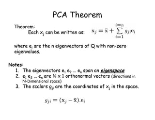
19. PCA Theorem
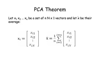
Let Q = X X
Let Q = X XT
T be the N x N matrix:
be the N x N matrix:
Notes:
Notes:
1.
1. Q is square
Q is square
2.
2. Q is symmetric
Q is symmetric
3.
3. Q is the
Q is the covariance
covariance matrix [aka scatter matrix]
matrix [aka scatter matrix]
4.
4. Q can be very large
Q can be very large (in vision, N is often the number of
(in vision, N is often the number of
pixels in an image!)
pixels in an image!)

20. PCA Theorem
where
where e
ei
i are the n eigenvectors of Q with non
are the n eigenvectors of Q with non-
-zero
zero
eigenvalues
eigenvalues.
.
Theorem:
Theorem:
Each
Each x
xj
j can be written as:
can be written as:
Notes:
Notes:
1.
1. The eigenvectors e
The eigenvectors e1
1 e
e2
2 …
… e
en
n span an
span an eigenspace
2. e1 e2 … en are N x 1 orthonormal vectors (directions in
N-Dimensional space)
3.
3. The scalars
The scalars g
gji
ji are the coordinates of
are the coordinates of x
xj
j in the space.
in the space.

21. Using PCA to Compress Data
• Expressing x in terms of e1 … en has not
changed the size of the data
• However, if the points are highly correlated
many of the coordinates of x will be zero or
closed to zero.
note: this means they lie in a
note: this means they lie in a
lower
lower-
-dimensional linear subspace
dimensional linear subspace

22. Using PCA to Compress Data
• Sort the eigenvectors ei according to
their eigenvalue:
•
•Assuming that
Assuming that
•
•Then
Then

23. PCA Example –STEP 1
http://kybele.psych.cornell.edu/~edelman/Psych-465-Spring-2003/PCA-tutorial.pdf
mean
mean
this becomes the
this becomes the
new origin of the
new origin of the
data from now on
data from now on
• DATA:
• x y
• 2.5 2.4
• 0.5 0.7
• 2.2 2.9
• 1.9 2.2
• 3.1 3.0
• 2.3 2.7
• 2 1.6
• 1 1.1
• 1.5 1.6
• 1.1 0.9

24. PCA Example –STEP 2
• Calculate the covariance matrix
cov = .616555556 .615444444
.615444444 .716555556
• since the non-diagonal elements in this
covariance matrix are positive, we should
expect that both the x and y variable
increase together.

25. PCA Example –STEP 3
• Calculate the eigenvectors and eigenvalues
of the covariance matrix
eigenvalues = .0490833989
1.28402771
eigenvectors = -.735178656 -.677873399
.677873399 -735178656

26. PCA Example –STEP 3
•eigenvectors are plotted
as diagonal dotted lines
on the plot.
•Note they are
perpendicular to each
other.
•Note one of the
eigenvectors goes through
the middle of the points,
like drawing a line of best
fit.
•The second eigenvector
gives us the other, less
important, pattern in the
data, that all the points
follow the main line, but
are off to the side of the
main line by some
amount.

27. PCA Example –STEP 4
• Feature Vector
FeatureVector = (eig1 eig2 eig3 … eign)
We can either form a feature vector with both of the
eigenvectors:
-.677873399 -.735178656
-.735178656 .677873399
or, we can choose to leave out the smaller, less
significant component and only have a single column:
- .677873399
- .735178656

28. PCA Example –STEP 5
• Deriving new data coordinates
FinalData = RowFeatureVector x RowZeroMeanData
RowFeatureVector is the matrix with the
eigenvectors in the columns transposed so that the
eigenvectors are now in the rows, with the most
significant eigenvector at the top
RowZeroMeanData is the mean-adjusted data
transposed, ie. the data items are in each
column, with each row holding a separate
dimension.
Note: his is essential
Note: his is essential Rotating
Rotating the coordinate axes
the coordinate axes
so higher
so higher-
-variance axes come first.
variance axes come first.

29. PCA Example –STEP 5

30. PCA Example : Approximation
• If we reduced the dimensionality,
obviously, when reconstructing the data
we would lose those dimensions we
chose to discard. In our example let us
assume that we considered only the x
dimension…

31. PCA Example : Final Approximation
2D point cloud
2D point cloud Approximation using
Approximation using
one eigenvector basis
one eigenvector basis

32. Another way of thinking
about Principal component
• direction of maximum variance in the input
space
• happens to be same as the principal
eigenvector of the covariance matrix

33. One-dimensional projection
find projection
find projection
that maximizes
that maximizes
variance
variance

34. Covariance to variance
• From the covariance, the variance of
any projection can be calculated.
• Let w be a unit vector
wT
x
 
2
 wT
x
2
 wT
Cw
 wiCijwj
ij


35. Maximizing variance
• Principal eigenvector of C
– the one with the largest eigenvalue.
w*
 argmax
w:w 1
wT
Cw
max C
  max
w:w 1
wT
Cw
 w*T
Cw*

36. Implementing PCA
• Need to find “first” k eigenvectors of Q:
Q is N x N (Again, N could be the number of pixels in
Q is N x N (Again, N could be the number of pixels in
an image. For a 256 x 256 image, N = 65536 !!)
an image. For a 256 x 256 image, N = 65536 !!)
Don
Don’
’t want to explicitly compute Q!!!!
t want to explicitly compute Q!!!!

37. Singular Value Decomposition
(SVD)
Any m x n matrix X can be written as the product of 3
Any m x n matrix X can be written as the product of 3
matrices:
matrices:
Where:
Where:
•
• U is m x m and its columns are
U is m x m and its columns are orthonormal
orthonormal vectors
vectors
•
• V is n x n and its columns are
V is n x n and its columns are orthonormal
orthonormal vectors
vectors
•
• D is m x n diagonal and its diagonal elements are called
D is m x n diagonal and its diagonal elements are called
the singular values of X, and are such that:
the singular values of X, and are such that:

1
1 ¸
¸ 
2
2 ¸
¸ …
… 
n
n ¸
¸ 0
0

38. SVD Properties
•
• The columns of U are the eigenvectors of XX
The columns of U are the eigenvectors of XXT
T
•
• The columns of V are the eigenvectors of X
The columns of V are the eigenvectors of XT
TX
X
•
• The squares of the diagonal elements of D are the
The squares of the diagonal elements of D are the
eigenvalues
eigenvalues of XX
of XXT
T and X
and XT
TX
X