Download to read offline

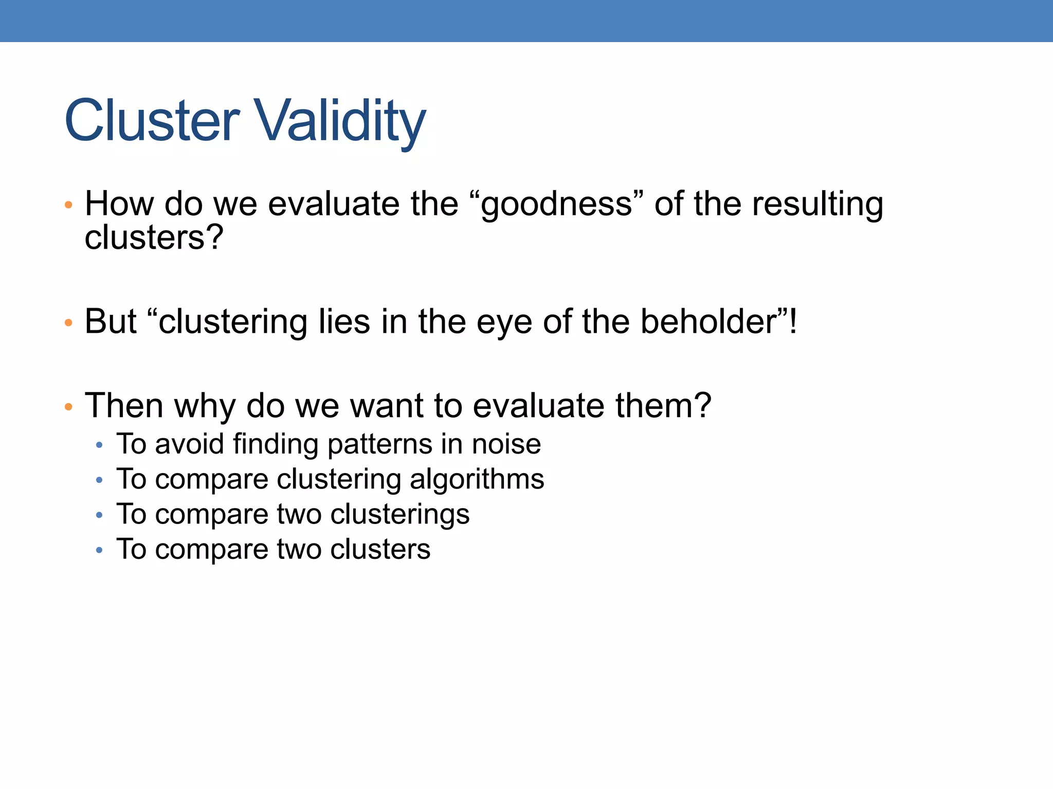
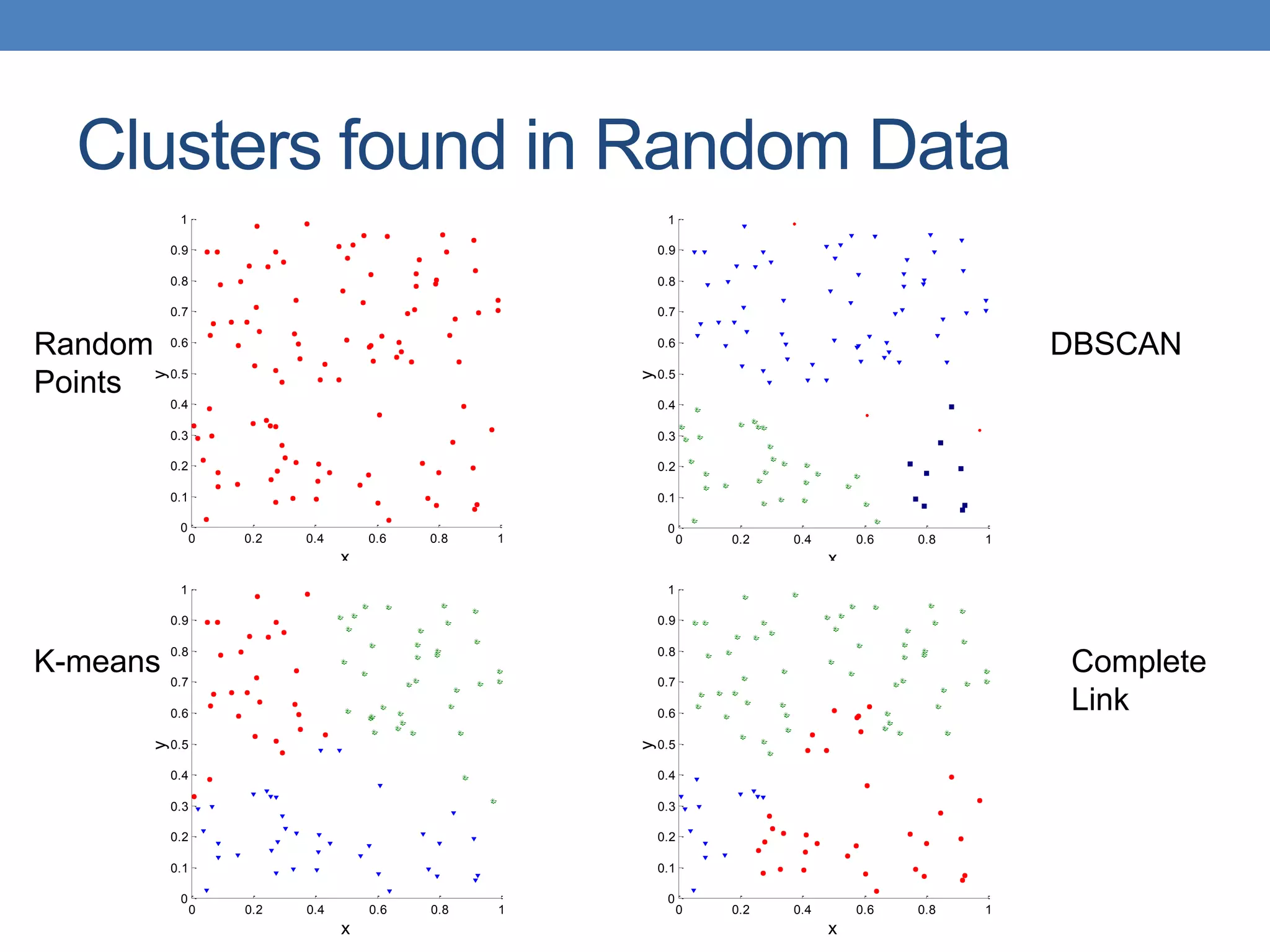
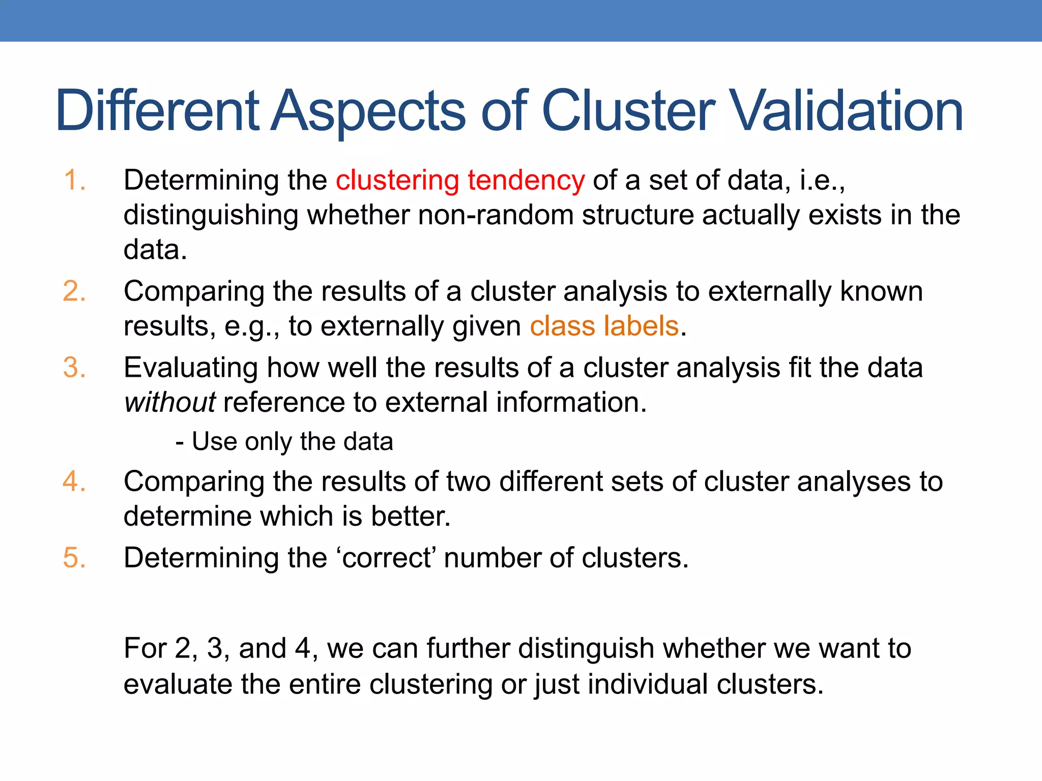
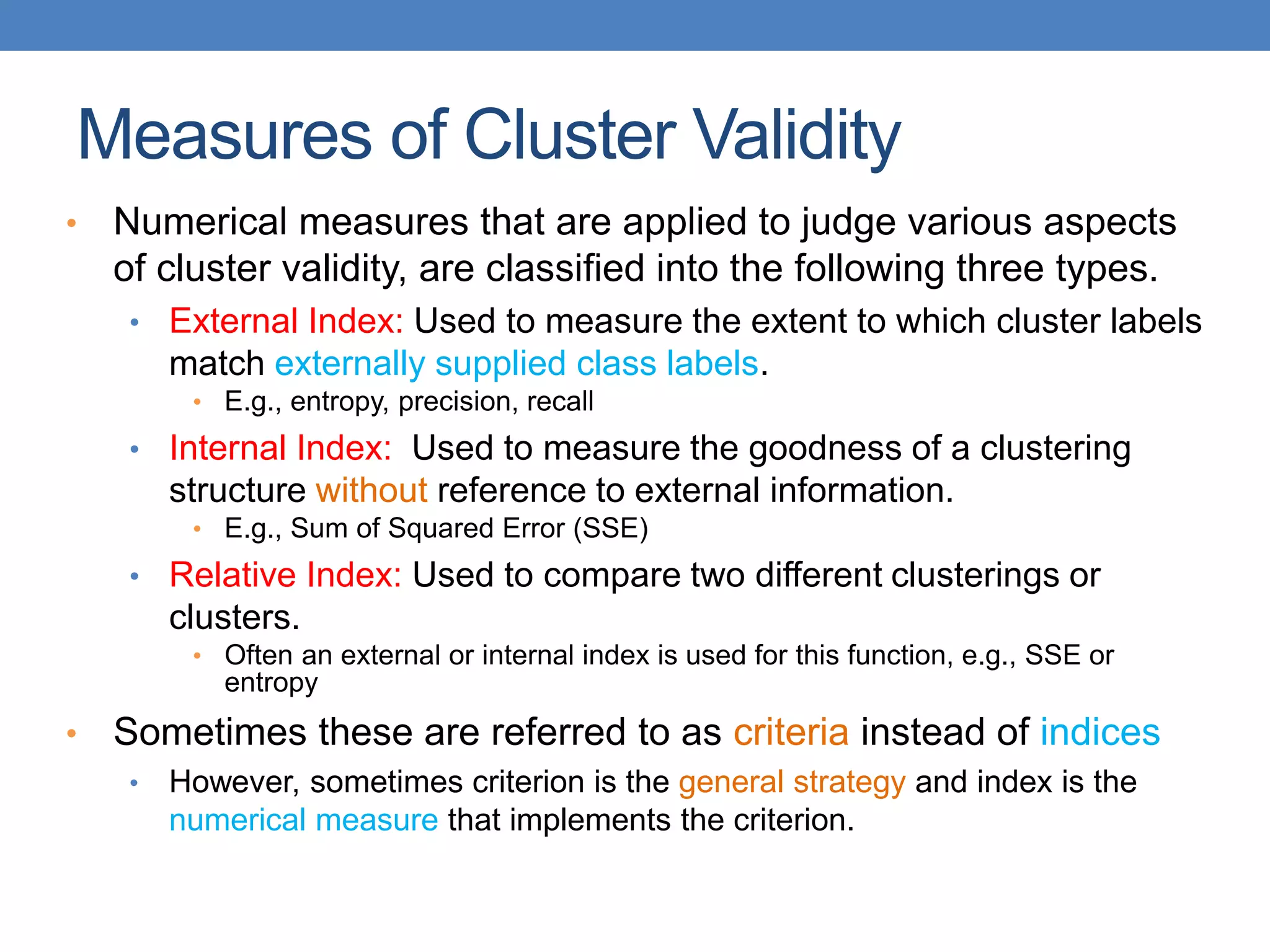
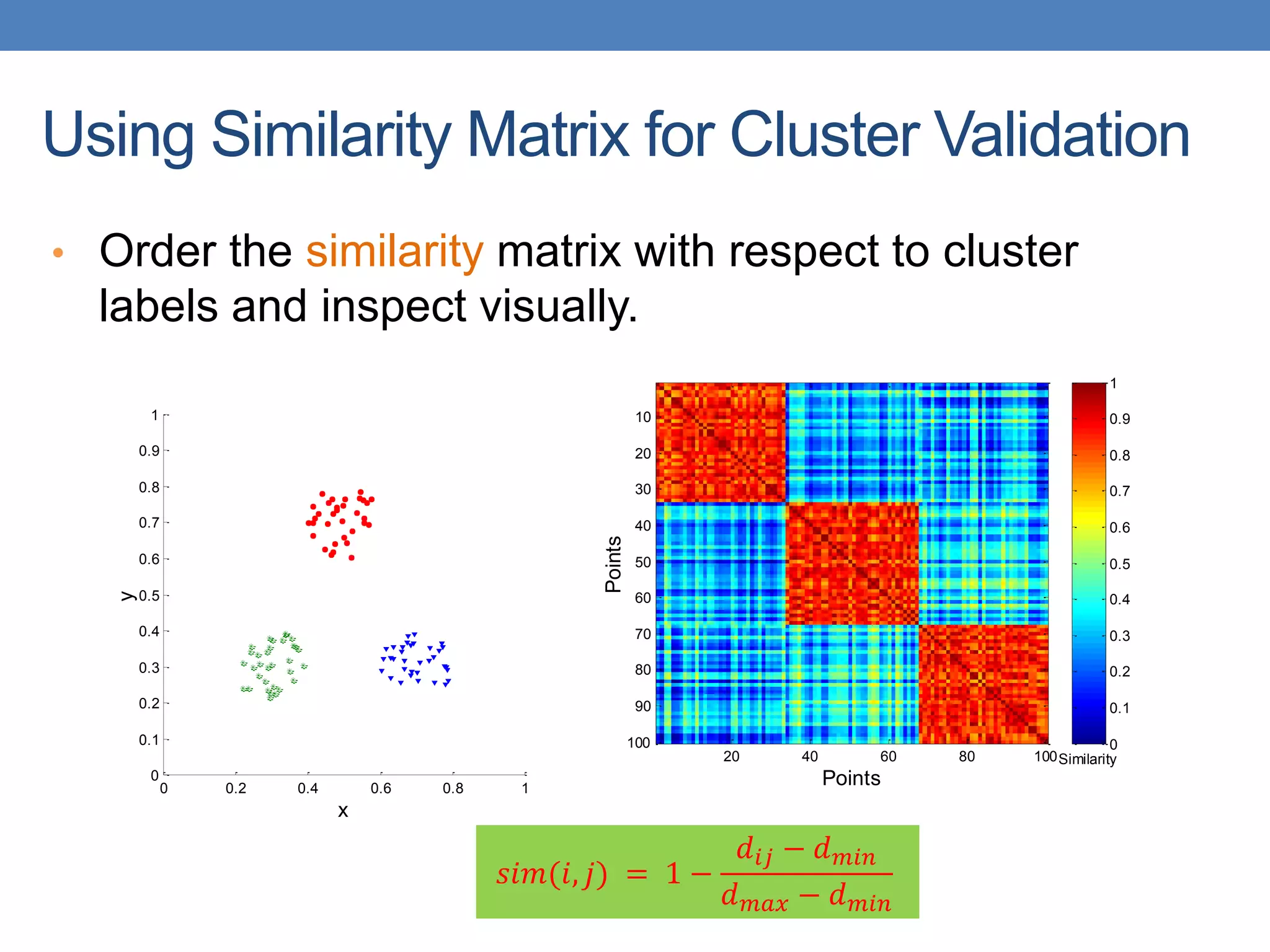
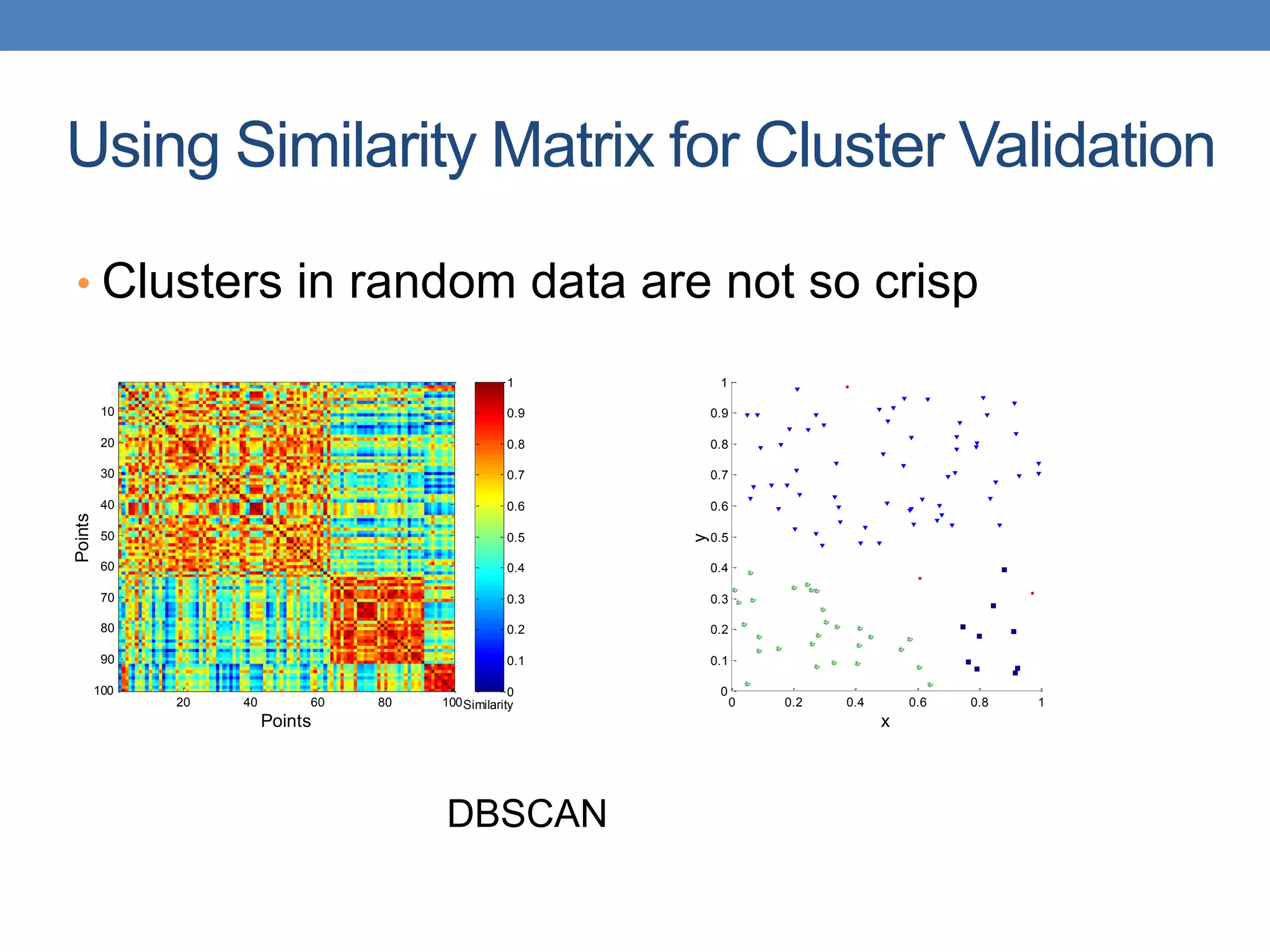
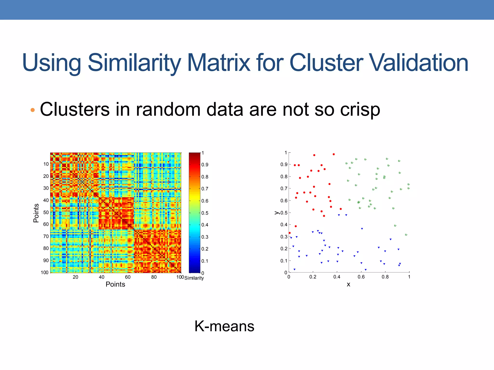
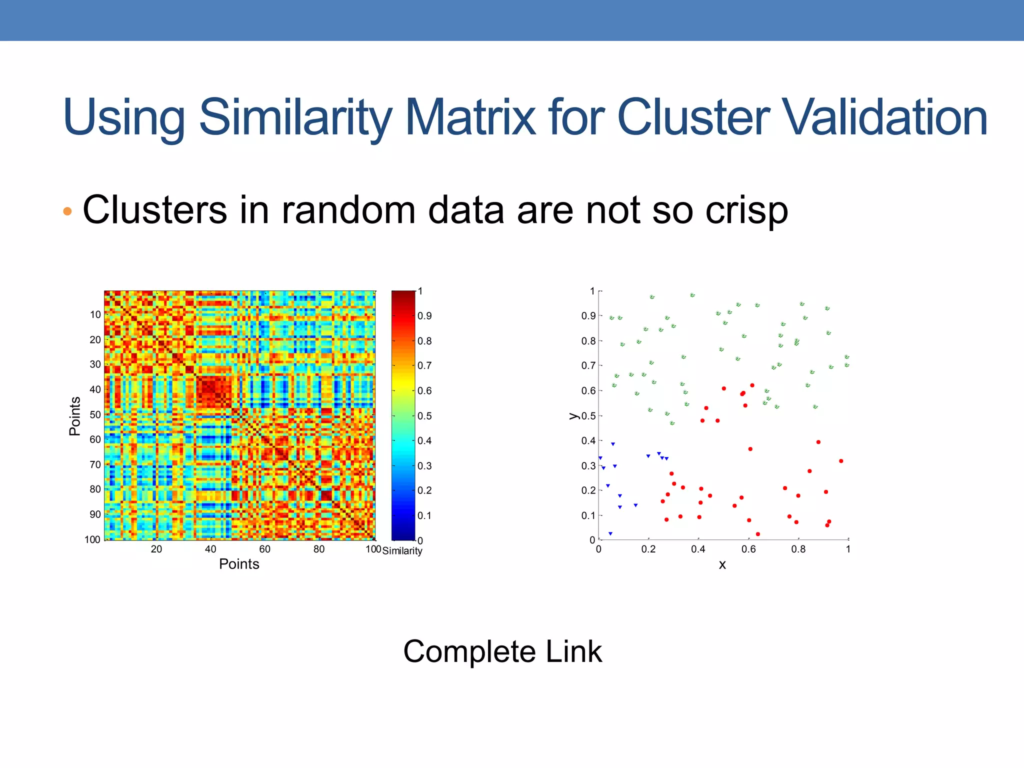
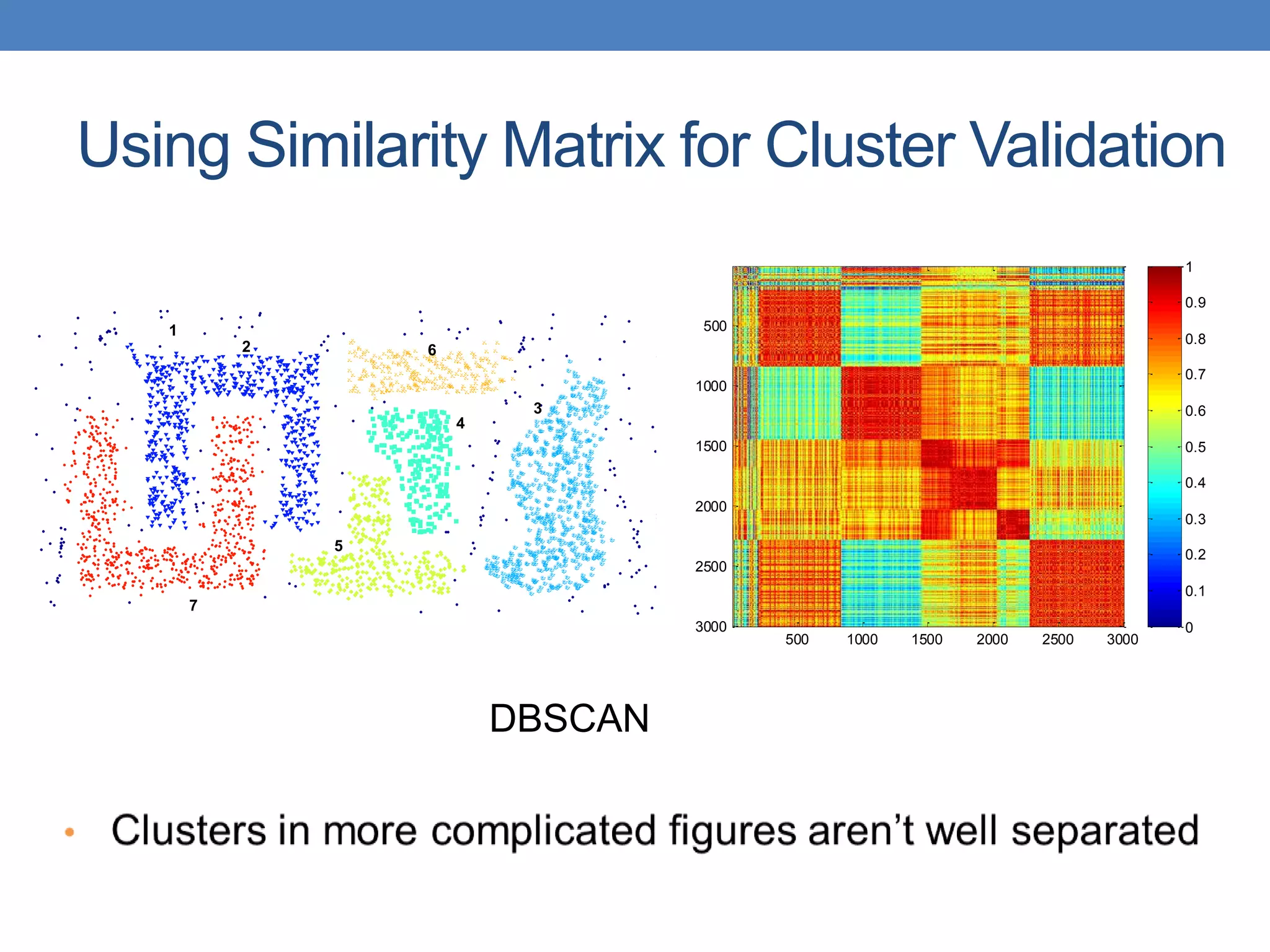
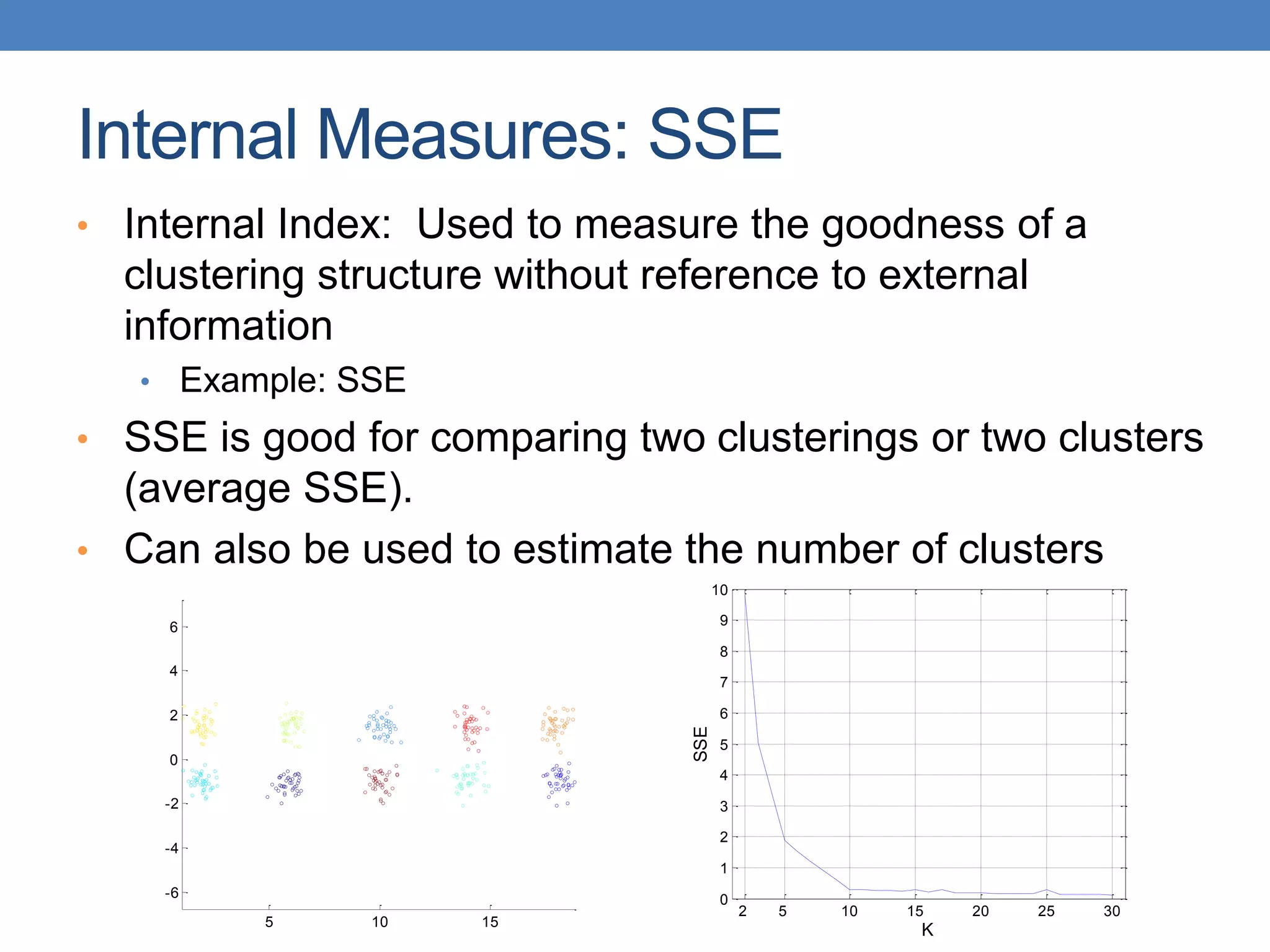
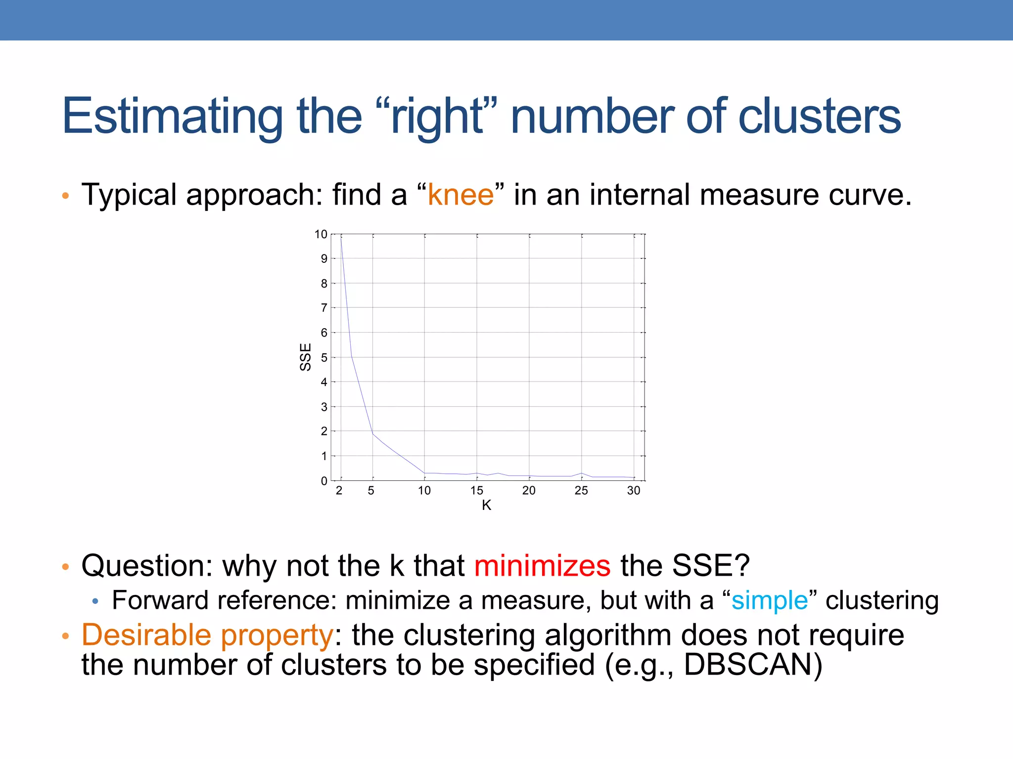
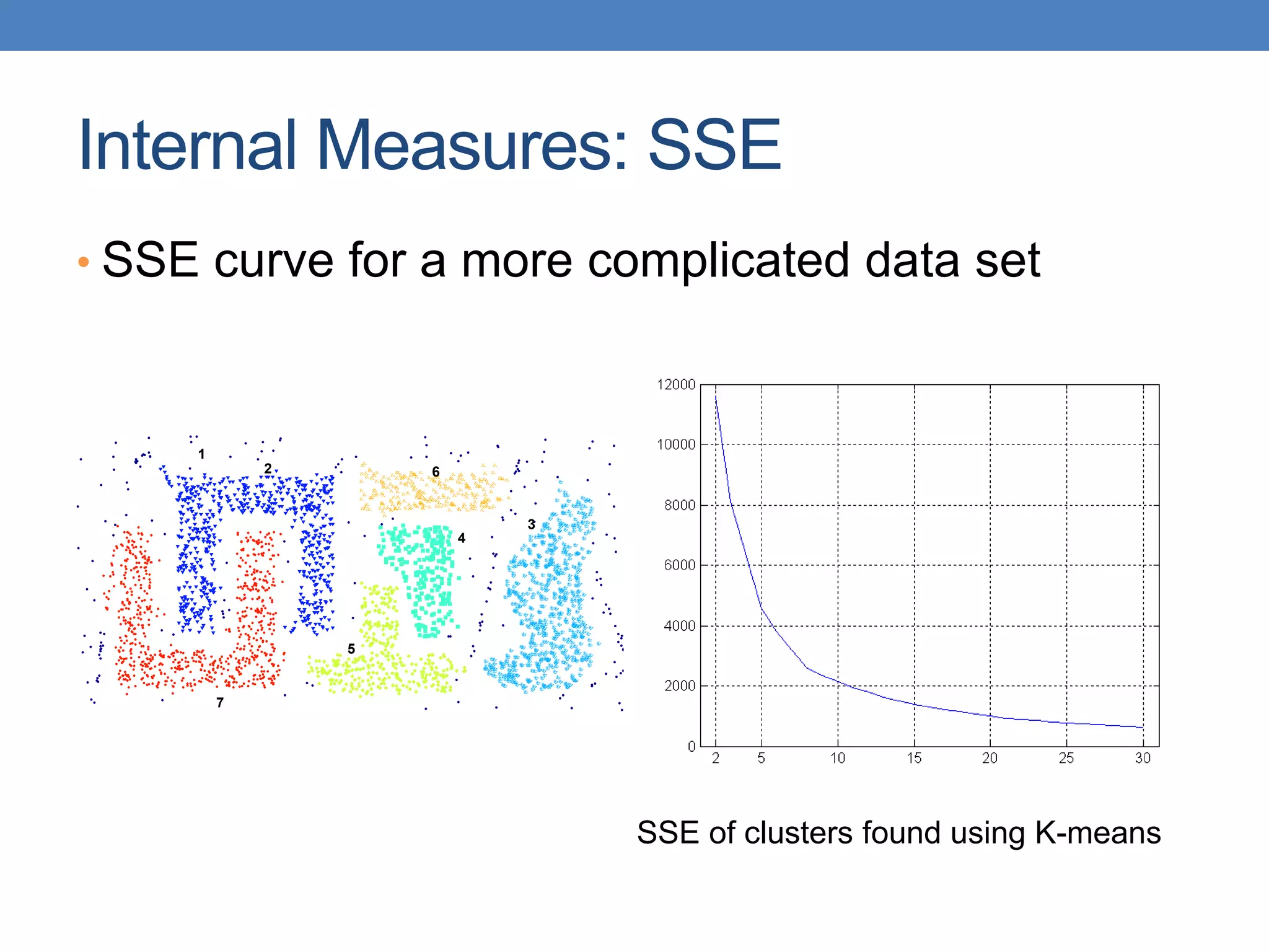
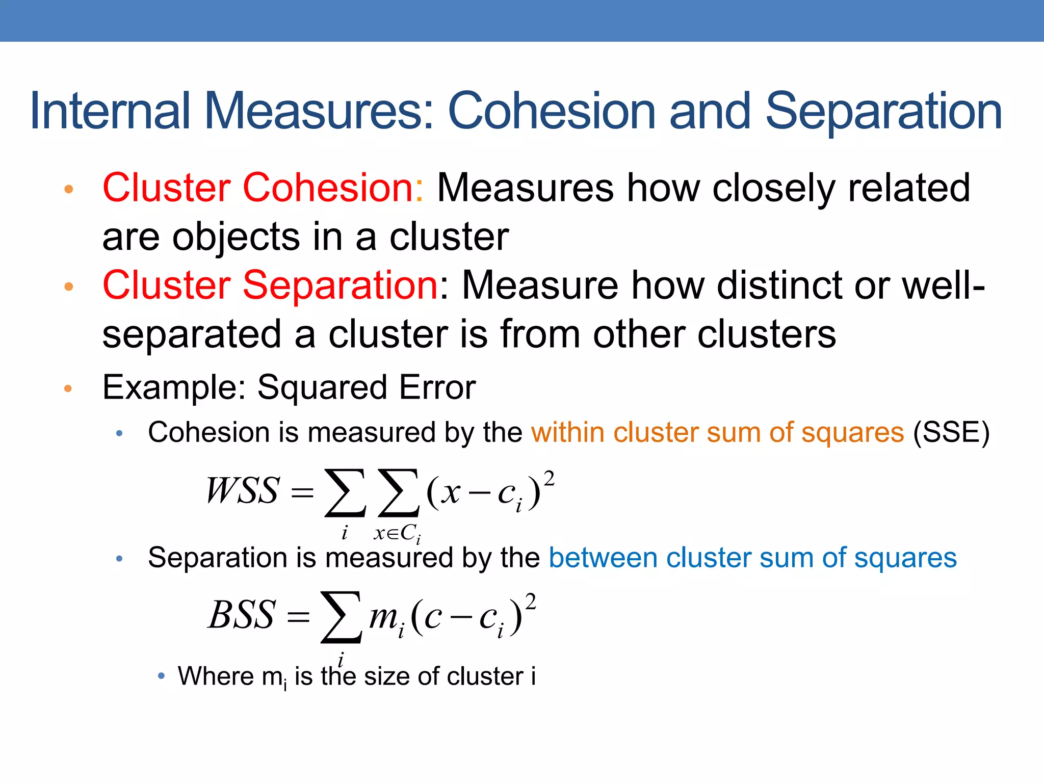
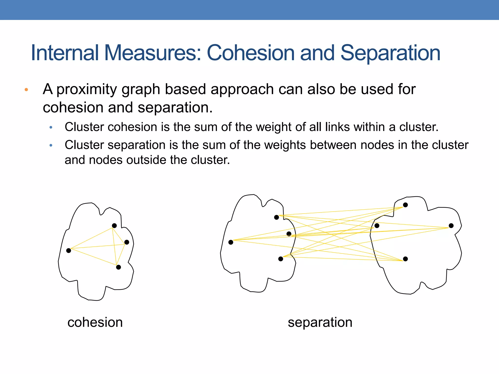
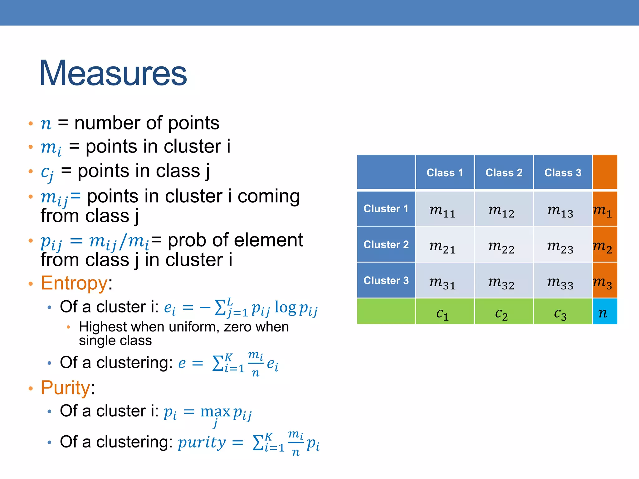
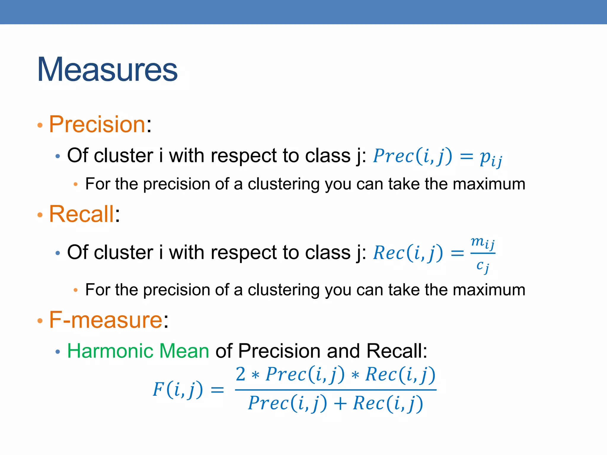
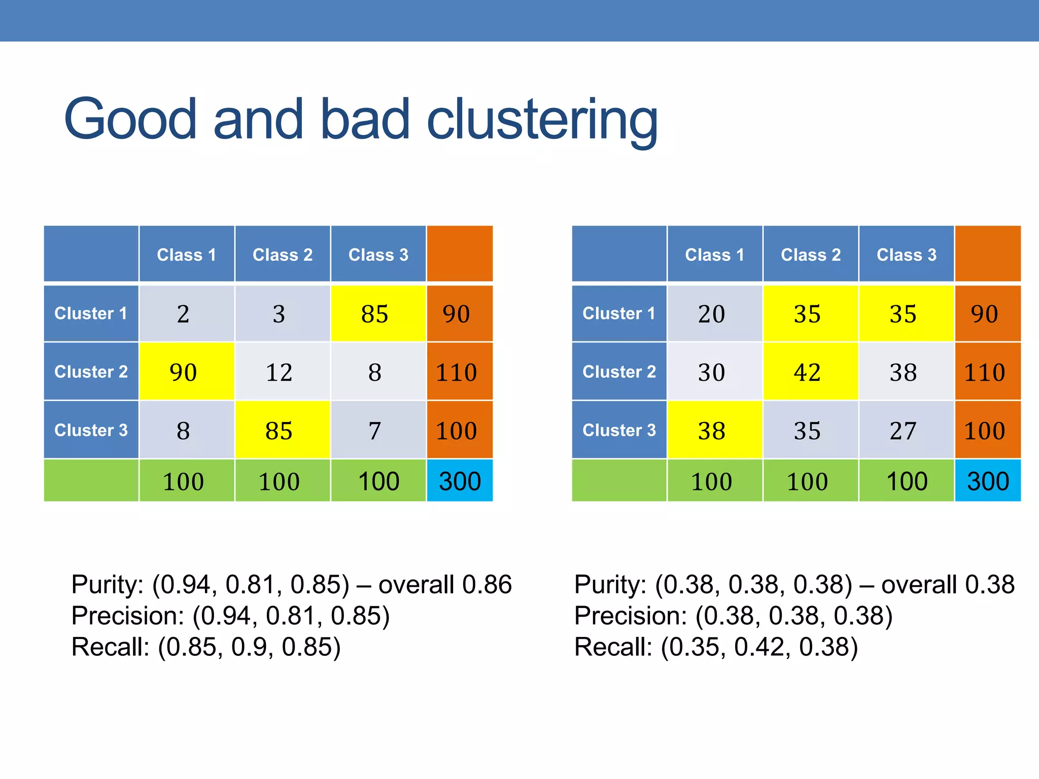
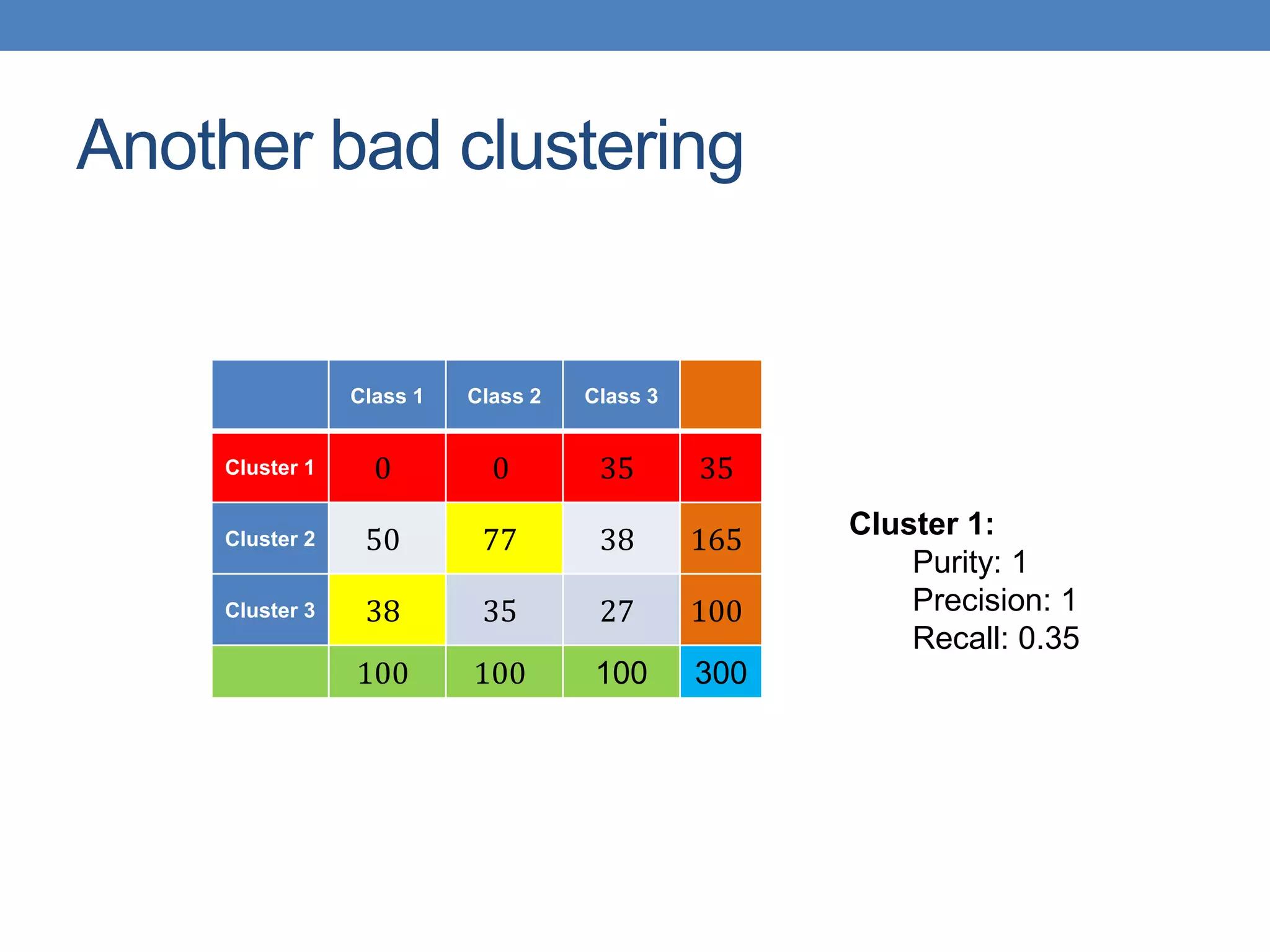
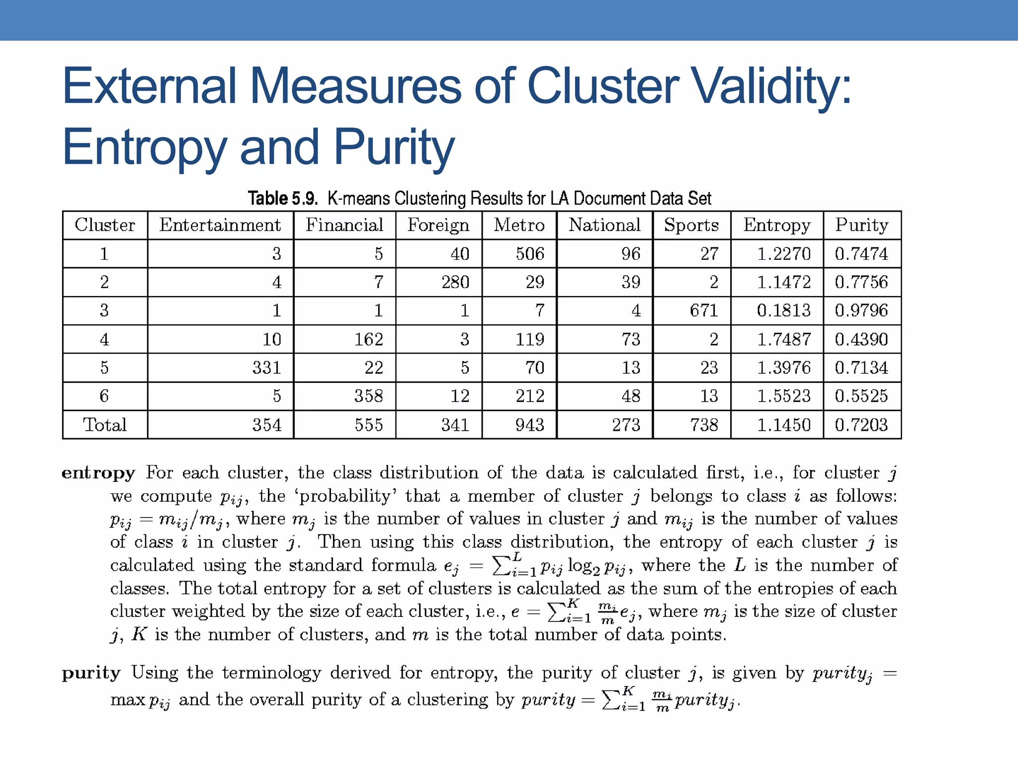

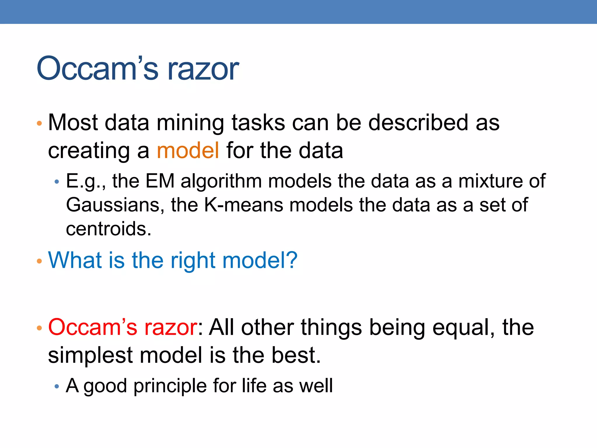
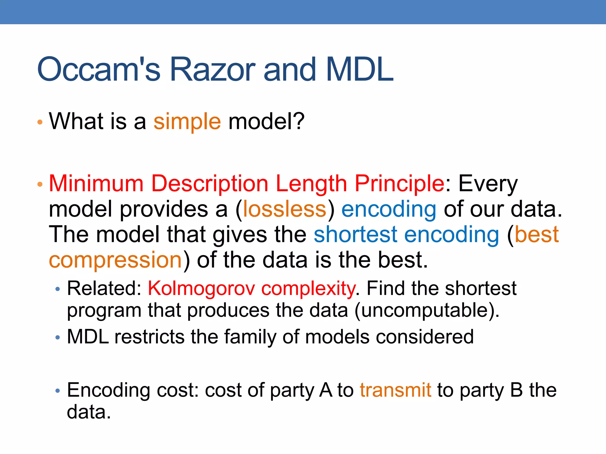
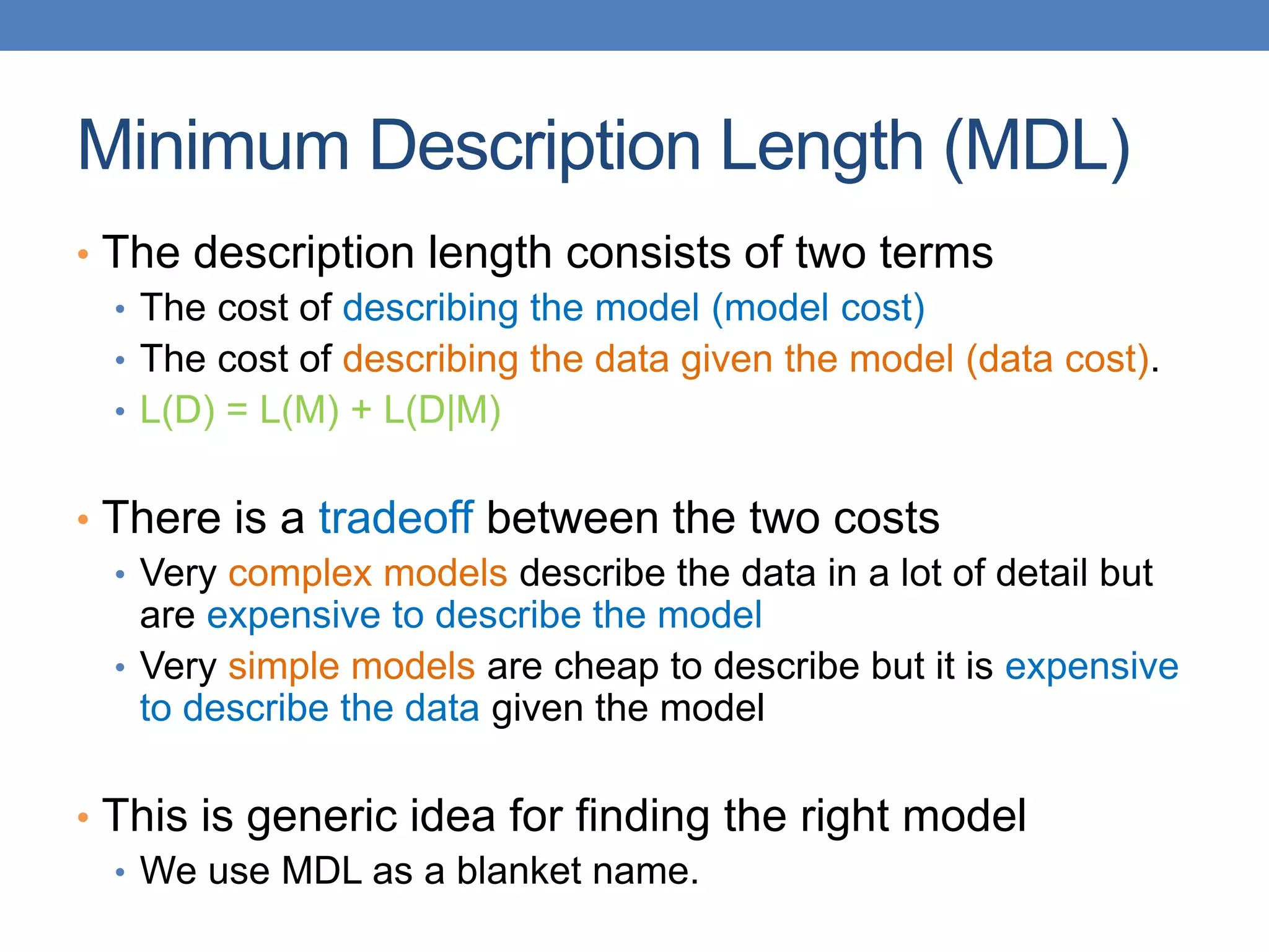
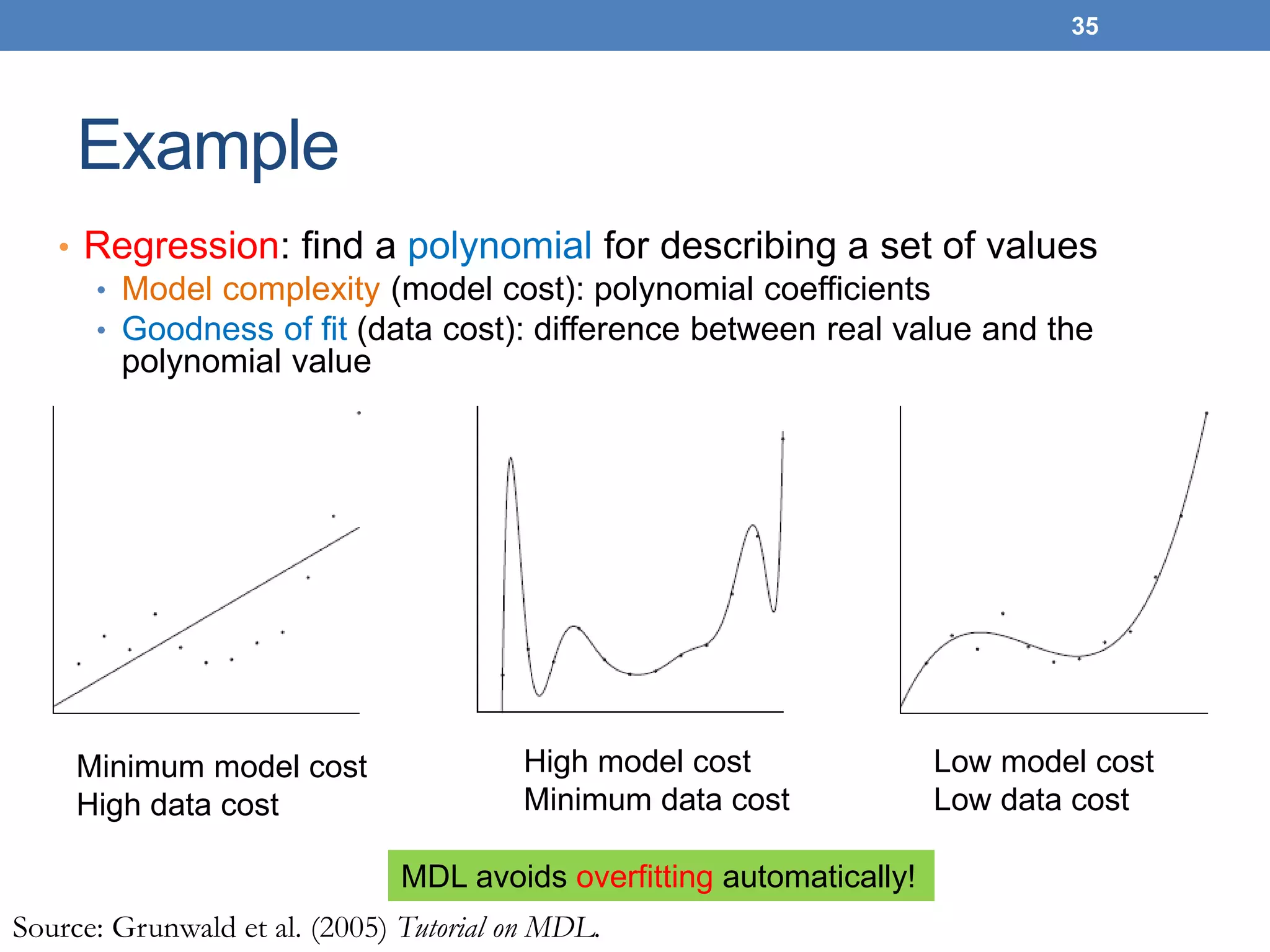
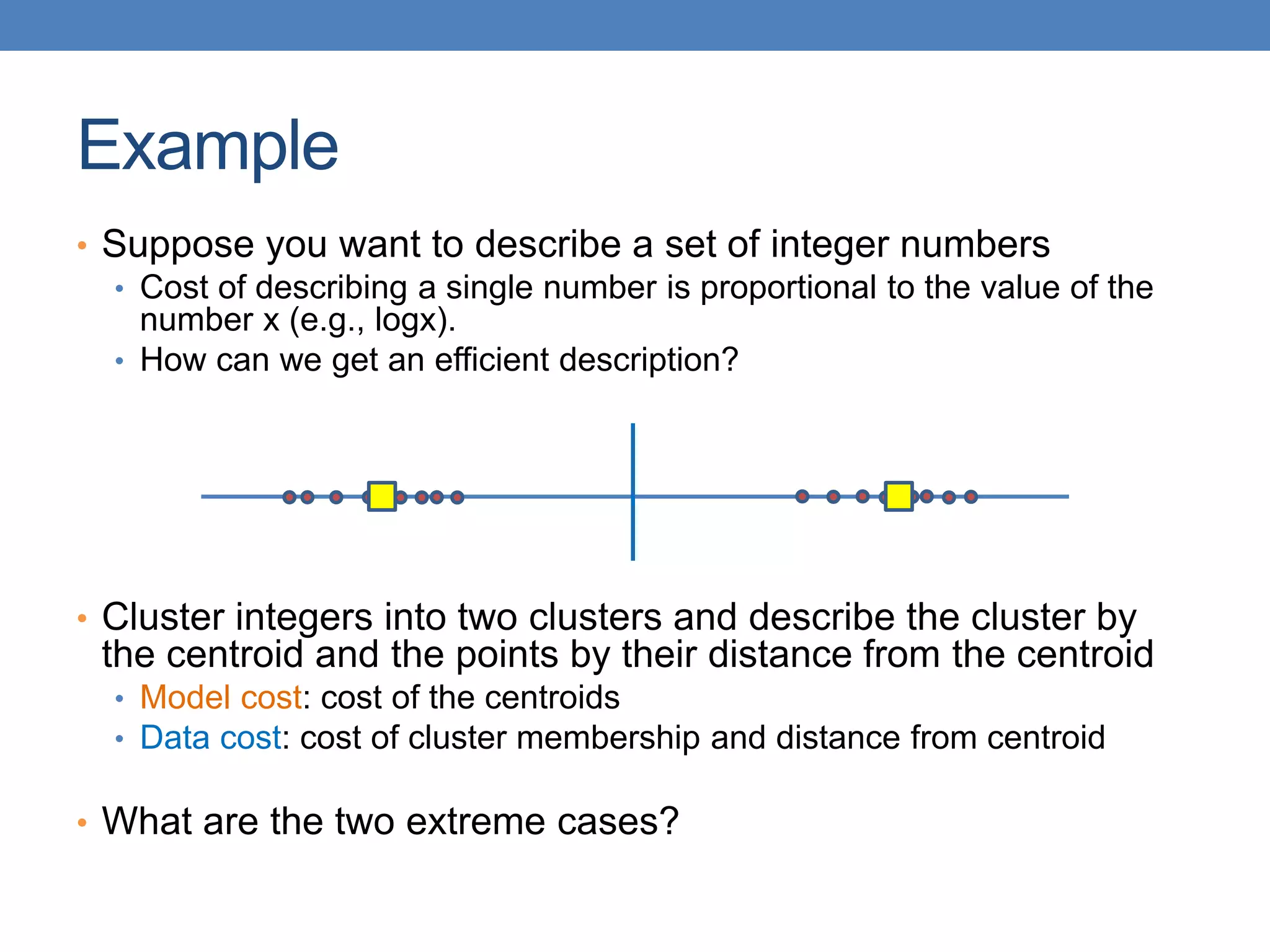
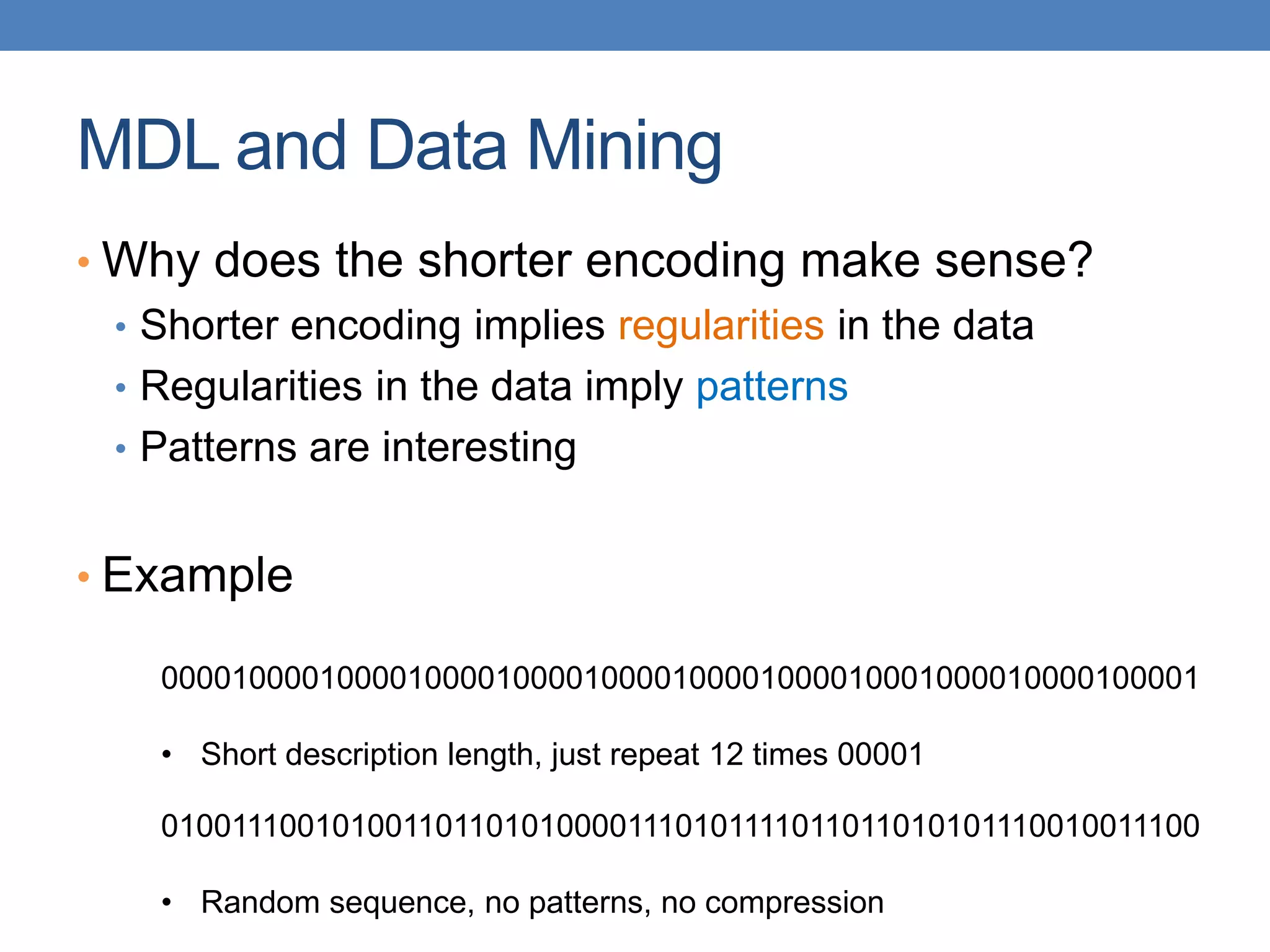
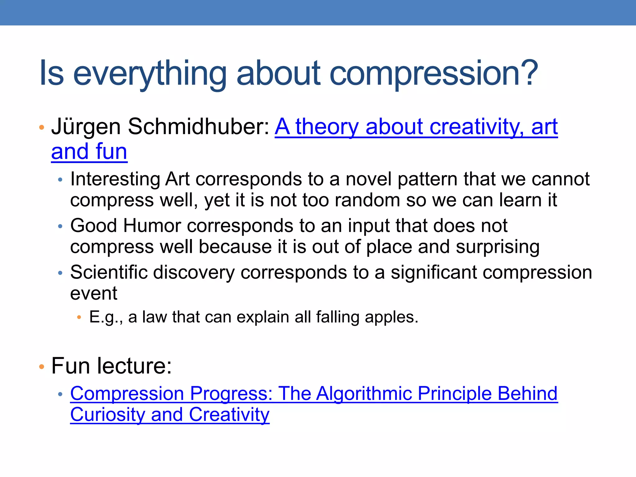
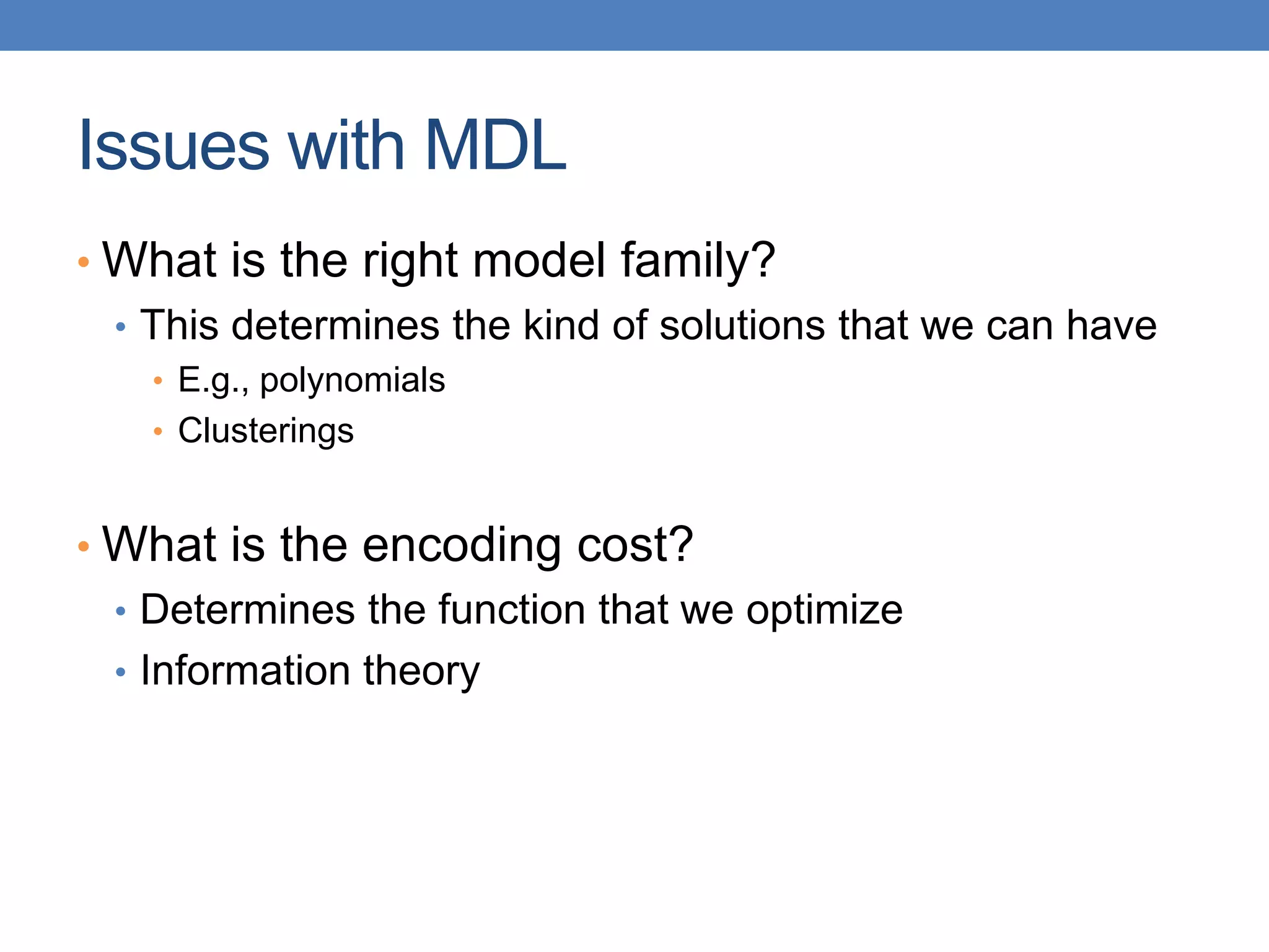

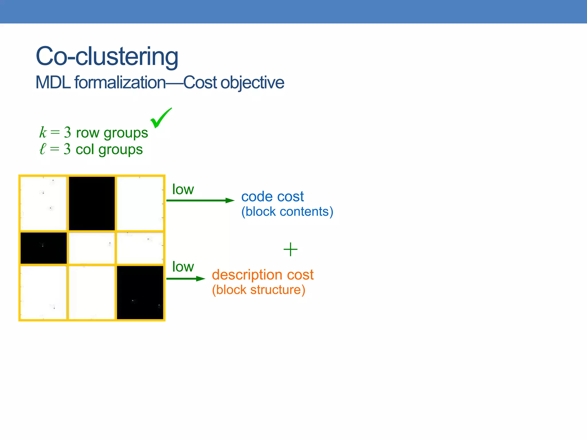
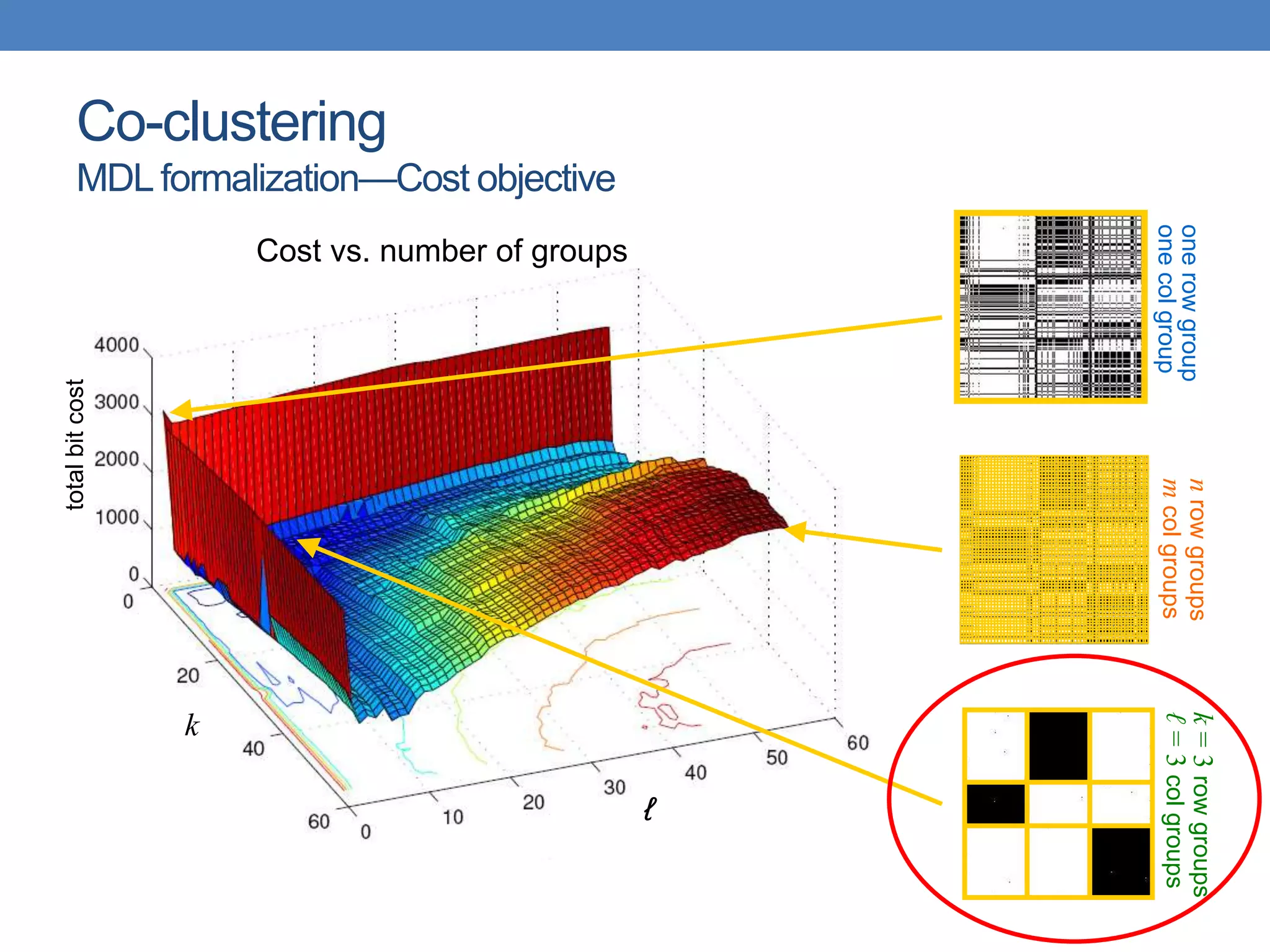
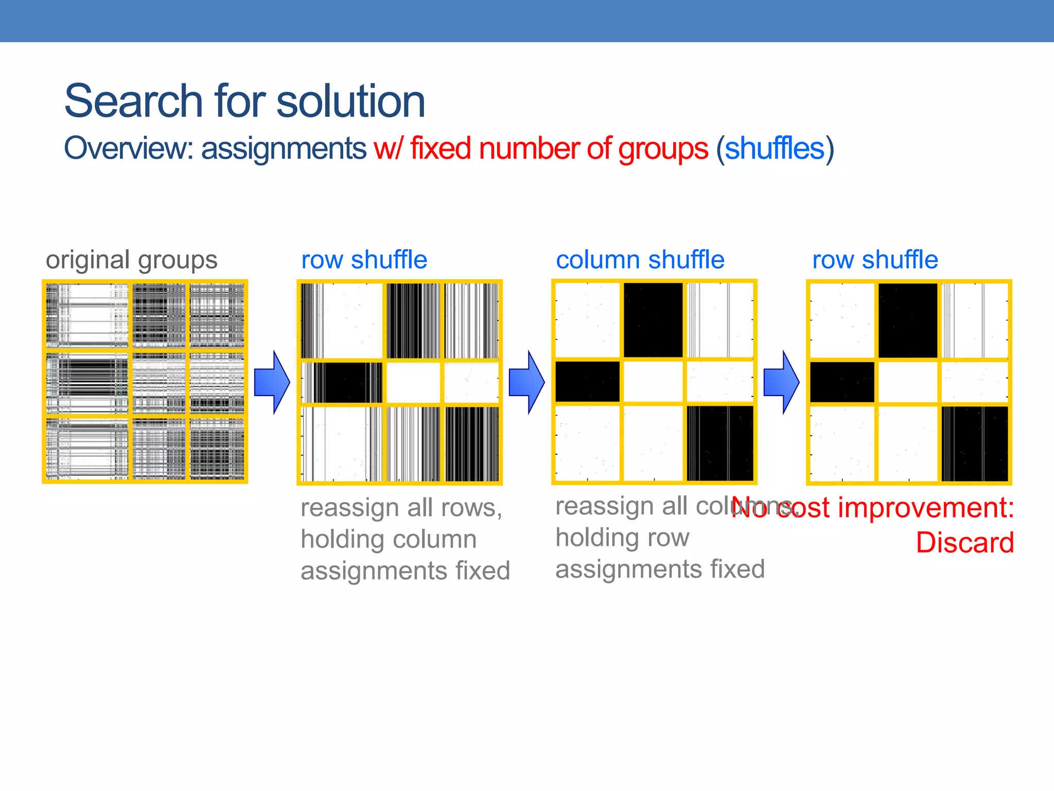

The lecture discusses clustering validation methods, emphasizing the importance of evaluating the quality of clusters to avoid identifying patterns in noise and to compare different clustering algorithms. It outlines various types of indices for evaluating cluster validity, including external, internal, and relative indices, along with techniques for measuring cohesion and separation among clusters. Additionally, it introduces the Minimum Description Length principle for selecting models based on information theory and model simplicity.