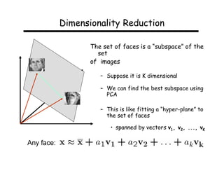
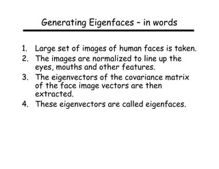
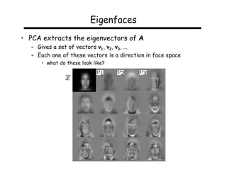
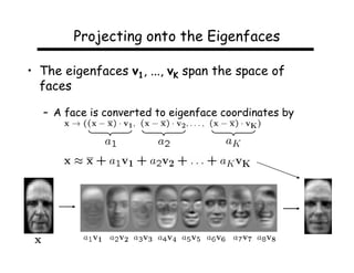
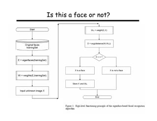
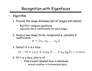
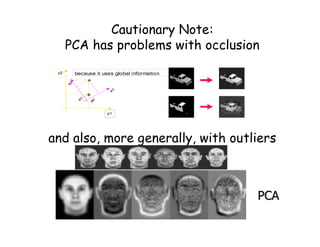
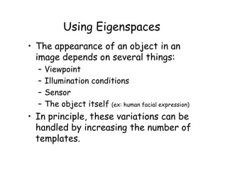
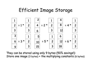
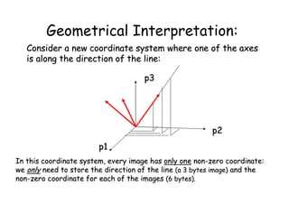
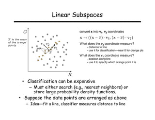
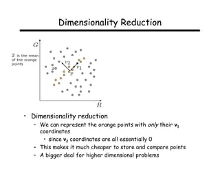
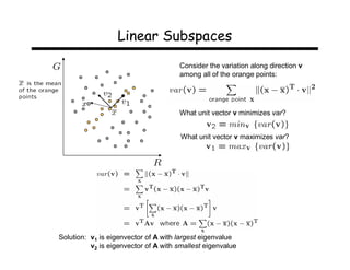
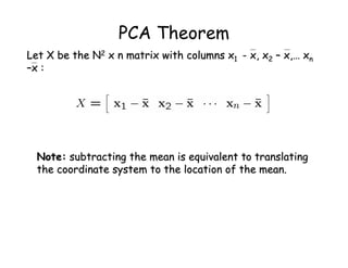
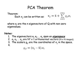
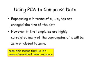
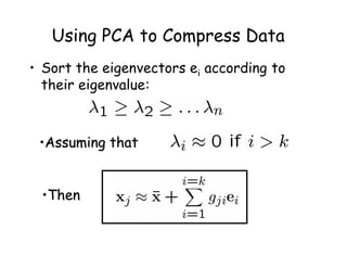
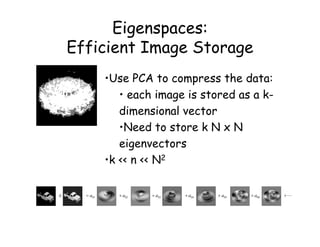
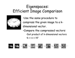
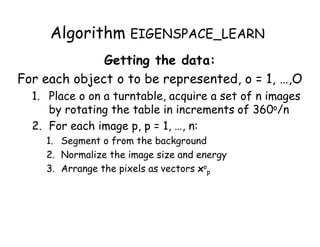
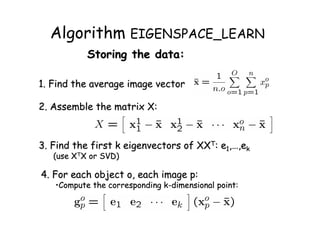
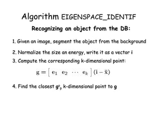
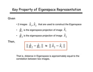
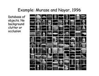
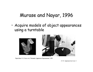
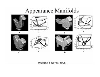
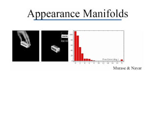
This document describes using principal component analysis (PCA) for object recognition from images. PCA is used to represent objects in an "eigenspace" where each object is represented by a point defined by its coordinates along the principal axes of variation among sample images. This provides an efficient representation that can handle variations in viewpoint, illumination, etc. by requiring fewer samples. The key steps are: (1) collect sample images and represent each as a high-dimensional vector, (2) compute eigenvectors of the sample covariance matrix to define the eigenspace, (3) project new images into this space for recognition.
Variational Autoencoders For Image GenerationJason Anderson
Meetup: https://www.meetup.com/Cognitive-Computing-Enthusiasts/events/260580395/
Video: https://www.youtube.com/watch?v=fnULFOyNZn8
Blog: http://www.compthree.com/blog/autoencoder/
Code: https://github.com/compthree/variational-autoencoder
An autoencoder is a machine learning algorithm that represents unlabeled high-dimensional data as points in a low-dimensional space. A variational autoencoder (VAE) is an autoencoder that represents unlabeled high-dimensional data as low-dimensional probability distributions. In addition to data compression, the randomness of the VAE algorithm gives it a second powerful feature: the ability to generate new data similar to its training data. For example, a VAE trained on images of faces can generate a compelling image of a new "fake" face. It can also map new features onto input data, such as glasses or a mustache onto the image of a face that initially lacks these features. In this talk, we will survey VAE model designs that use deep learning, and we will implement a basic VAE in TensorFlow. We will also demonstrate the encoding and generative capabilities of VAEs and discuss their industry applications.
Robust Control of Uncertain Switched Linear Systems based on Stochastic Reach...Leo Asselborn
This presentation proposes an approach to algorithmically synthesize control strategies for
set-to-set transitions of uncertain discrete-time switched linear systems based on a combination
of tree search and reachable set computations in a stochastic setting. For given Gaussian
distributions of the initial states and disturbances, state sets wich are reachable to a chosen
confidence level under the effect of time-variant hybrid control laws are computed by using
principles of the ellipsoidal calculus. The proposed algorithm iterates over sequences of the
discrete states and LMI-constrained semi-definite programming (SDP) problems to compute
stabilizing controllers, while polytopic input constraints are considered. An example for illustration is included.
Animashree Anandkumar, Electrical Engineering and CS Dept, UC Irvine at MLcon...MLconf
Anima Anandkumar is a faculty at the EECS Dept. at U.C.Irvine since August 2010. Her research interests are in the area of large-scale machine learning and high-dimensional statistics. She received her B.Tech in Electrical Engineering from IIT Madras in 2004 and her PhD from Cornell University in 2009. She has been a visiting faculty at Microsoft Research New England in 2012 and a postdoctoral researcher at the Stochastic Systems Group at MIT between 2009-2010. She is the recipient of the Microsoft Faculty Fellowship, ARO Young Investigator Award, NSF CAREER Award, and IBM Fran Allen PhD fellowship.
Principal Components Analysis, Calculation and VisualizationMarjan Sterjev
The article explains dimension reduction principles, PCA algorithm and mathematics behind. The PCA calculation and data projection is demonstrated in R, Python and Apache Spark. Finally the results are visualized with D3.js.
Deep learning paper review ppt sourece -Direct clr taeseon ryu
딥러닝 이미지 분류 테스크에서는 Self-Supervision 학습 방법이 있습니다. 레이블이 없는 상태에서 context prediction 이나 jigsaw puzzle과 같은 방법으로 학습시키는 방법이지만 이러한 self-supervision 테스크에는 모든 차원에 분포하지 않고 특정 부분 차원으로만 학습이 되는 Dimensional Collapse 라는 고질적인 문제를 일으킵니다. Self-supervision 중 positive pair는 가깝게, 그리고 negative pair는 서로 멀어지게 학습을 시키는 Contrastive Learning 이 있습니다. 이로인해 Dimensional Collapse에 강인할 것 이라고 직관적으로 생각이 들지만, 그렇지 않았습니다. 이러한 문제를 해결하기 위해 등장한 Direct CLR이라는 방법론을 소개드립니다.
논문의 배경부터 Direct CLR논문에 대한 디테일한 설명까지,
펀디멘탈팀의 이재윤님이 자세한 리뷰 도와주셨습니다.
오늘도 많은 관심 미리 감사드립니다 !
Kernel based models for geo- and environmental sciences- Alexei Pozdnoukhov –...Beniamino Murgante
Kernel based models for geo- and environmental sciences- Alexei Pozdnoukhov – National Centre for Geocomputation, National University of Ireland , Maynooth (Ireland)
Intelligent Analysis of Environmental Data (S4 ENVISA Workshop 2009)
Animashree Anandkumar, Electrical Engineering and CS Dept, UC Irvine at MLcon...MLconf
Tensor Methods: A New Paradigm for Training Probabilistic Models and Feature Learning: Tensors are rich structures for modeling complex higher order relationships in data rich domains such as social networks, computer vision, internet of things, and so on. Tensor decomposition methods are embarrassingly parallel and scalable to enormous datasets. They are guaranteed to converge to the global optimum and yield consistent estimates of parameters for many probabilistic models such as topic models, community models, hidden Markov models, and so on. I will show the results of these methods for learning topics from text data, communities in social networks, disease hierarchies from healthcare records, cell types from mouse brain data, etc. I will also demonstrate how tensor methods can yield rich discriminative features for classification tasks and can serve as an alternative method for training neural networks.
In order to be able to visulaize the data, or simply to speed up the process of learning without loosing the important features, we apply dimensionality reduction. methods.
We will talk about 2 methods: PCA and manifold.
[Notebook](https://colab.research.google.com/drive/1_ksjf1K49dUA8XtyDGoL5V3JEajHvFHb)
https://telecombcn-dl.github.io/2017-dlai/
Deep learning technologies are at the core of the current revolution in artificial intelligence for multimedia data analysis. The convergence of large-scale annotated datasets and affordable GPU hardware has allowed the training of neural networks for data analysis tasks which were previously addressed with hand-crafted features. Architectures such as convolutional neural networks, recurrent neural networks or Q-nets for reinforcement learning have shaped a brand new scenario in signal processing. This course will cover the basic principles of deep learning from both an algorithmic and computational perspectives.
Presentation of my NSERC-USRA funded summer research project given at the Canadian Undergraduate Mathematics Conference (CUMC) 2014.
Please refer to the project site: http://jessebett.com/Radial-Basis-Function-USRA/
Image Restoration UsingNonlocally Centralized Sparse Representation and histo...IJERA Editor
Due to the degradation of observed image the noisy, blurred, distorted image can be occurred .To restore the image informationby conventional modelsmay not be accurate enough for faithful reconstruction of the original image. I propose the sparse representations to improve the performance of based image restoration. In this method the sparse coding noise is added for image restoration, due to this image restoration the sparse coefficients of original image can be detected. The so-called nonlocally centralized sparse representation (NCSR) model is as simple as the standard sparse representation model, fordenoising the image here we use the histogram clipping method by using histogram based sparse representation to effectively reduce the noise and also implement the TMR filter for Quality image. Various types of image restoration problems, including denoising, deblurring and super-resolution, validate the generality and state-of-the-art performance of the proposed algorithm.
Animashree Anandkumar, Electrical Engineering and CS Dept, UC Irvine at MLcon...MLconf
Anima Anandkumar is a faculty at the EECS Dept. at U.C.Irvine since August 2010. Her research interests are in the area of large-scale machine learning and high-dimensional statistics. She received her B.Tech in Electrical Engineering from IIT Madras in 2004 and her PhD from Cornell University in 2009. She has been a visiting faculty at Microsoft Research New England in 2012 and a postdoctoral researcher at the Stochastic Systems Group at MIT between 2009-2010. She is the recipient of the Microsoft Faculty Fellowship, ARO Young Investigator Award, NSF CAREER Award, and IBM Fran Allen PhD fellowship.
Principal Components Analysis, Calculation and VisualizationMarjan Sterjev
The article explains dimension reduction principles, PCA algorithm and mathematics behind. The PCA calculation and data projection is demonstrated in R, Python and Apache Spark. Finally the results are visualized with D3.js.
Deep learning paper review ppt sourece -Direct clr taeseon ryu
딥러닝 이미지 분류 테스크에서는 Self-Supervision 학습 방법이 있습니다. 레이블이 없는 상태에서 context prediction 이나 jigsaw puzzle과 같은 방법으로 학습시키는 방법이지만 이러한 self-supervision 테스크에는 모든 차원에 분포하지 않고 특정 부분 차원으로만 학습이 되는 Dimensional Collapse 라는 고질적인 문제를 일으킵니다. Self-supervision 중 positive pair는 가깝게, 그리고 negative pair는 서로 멀어지게 학습을 시키는 Contrastive Learning 이 있습니다. 이로인해 Dimensional Collapse에 강인할 것 이라고 직관적으로 생각이 들지만, 그렇지 않았습니다. 이러한 문제를 해결하기 위해 등장한 Direct CLR이라는 방법론을 소개드립니다.
논문의 배경부터 Direct CLR논문에 대한 디테일한 설명까지,
펀디멘탈팀의 이재윤님이 자세한 리뷰 도와주셨습니다.
오늘도 많은 관심 미리 감사드립니다 !
Kernel based models for geo- and environmental sciences- Alexei Pozdnoukhov –...Beniamino Murgante
Kernel based models for geo- and environmental sciences- Alexei Pozdnoukhov – National Centre for Geocomputation, National University of Ireland , Maynooth (Ireland)
Intelligent Analysis of Environmental Data (S4 ENVISA Workshop 2009)
Animashree Anandkumar, Electrical Engineering and CS Dept, UC Irvine at MLcon...MLconf
Tensor Methods: A New Paradigm for Training Probabilistic Models and Feature Learning: Tensors are rich structures for modeling complex higher order relationships in data rich domains such as social networks, computer vision, internet of things, and so on. Tensor decomposition methods are embarrassingly parallel and scalable to enormous datasets. They are guaranteed to converge to the global optimum and yield consistent estimates of parameters for many probabilistic models such as topic models, community models, hidden Markov models, and so on. I will show the results of these methods for learning topics from text data, communities in social networks, disease hierarchies from healthcare records, cell types from mouse brain data, etc. I will also demonstrate how tensor methods can yield rich discriminative features for classification tasks and can serve as an alternative method for training neural networks.
In order to be able to visulaize the data, or simply to speed up the process of learning without loosing the important features, we apply dimensionality reduction. methods.
We will talk about 2 methods: PCA and manifold.
[Notebook](https://colab.research.google.com/drive/1_ksjf1K49dUA8XtyDGoL5V3JEajHvFHb)
https://telecombcn-dl.github.io/2017-dlai/
Deep learning technologies are at the core of the current revolution in artificial intelligence for multimedia data analysis. The convergence of large-scale annotated datasets and affordable GPU hardware has allowed the training of neural networks for data analysis tasks which were previously addressed with hand-crafted features. Architectures such as convolutional neural networks, recurrent neural networks or Q-nets for reinforcement learning have shaped a brand new scenario in signal processing. This course will cover the basic principles of deep learning from both an algorithmic and computational perspectives.
Presentation of my NSERC-USRA funded summer research project given at the Canadian Undergraduate Mathematics Conference (CUMC) 2014.
Please refer to the project site: http://jessebett.com/Radial-Basis-Function-USRA/
Image Restoration UsingNonlocally Centralized Sparse Representation and histo...IJERA Editor
Due to the degradation of observed image the noisy, blurred, distorted image can be occurred .To restore the image informationby conventional modelsmay not be accurate enough for faithful reconstruction of the original image. I propose the sparse representations to improve the performance of based image restoration. In this method the sparse coding noise is added for image restoration, due to this image restoration the sparse coefficients of original image can be detected. The so-called nonlocally centralized sparse representation (NCSR) model is as simple as the standard sparse representation model, fordenoising the image here we use the histogram clipping method by using histogram based sparse representation to effectively reduce the noise and also implement the TMR filter for Quality image. Various types of image restoration problems, including denoising, deblurring and super-resolution, validate the generality and state-of-the-art performance of the proposed algorithm.
Face Recognition using PCA-Principal Component Analysis using MATLABSindhi Madhuri
It describes about a biometric technique to recognize people at a particular environment using MATLAB. It simply forms EIGENFACES and compares Principal components instead of each and every pixel of an image.
Image generation. Gaussian models for human faces, limits and relations with linear neural networks. Generative adversarial networks (GANs), generators, discrinators, adversarial loss and two player games. Convolutional GAN and image arithmetic. Super-resolution. Nearest-neighbor, bilinear and bicubic interpolation. Image sharpening. Linear inverse problems, Tikhonov and Total-Variation regularization. Super-Resolution CNN, VDSR, Fast SRCNN, SRGAN, perceptual, adversarial and content losses. Style transfer: Gatys model, content loss and style loss.
Efficient Variable Size Template Matching Using Fast Normalized Cross Correla...Gurbinder Gill
In this presentation we propose the parallel implementation of template matching using Full Search using NCC as a measure using the concept of pre-computed sum-tables referred to as FNCC for high resolution images on NVIDIA’s Graphics Processing Units (GP-GPU’s)
3. Hypotheses fromTemplate Matching
•Place the template at every
location on the given image.
•Compare the pixel values in
the template with the pixel
values in the underlying region
of the image.
•If a “good” match is found, •Possible measures are: SSD,
announce that the object is SAD, Cross-correlation,
Normalized Cross-correlation,
present in the image. max difference, etc.
4. Limitations of Template Matching
• If the object appears scaled, rotated, or
skewed on the image, the match will not
be good.
5. Solution:
• Search for the template and possible
transformations of the template:
Not very efficient! (but doable …)
6. Using Eigenspaces
• The appearance of an object in an
image depends on several things:
– Viewpoint
– Illumination conditions
– Sensor
– The object itself (ex: human facial expression)
• In principle, these variations can be
handled by increasing the number of
templates.
7. Eigenspaces:
Using multiple templates
•The number of templates can grow very fast!
•We need:
•An efficient way to store templates
•An efficient way to search for matches
•Observation: while each template is different,
there exist many similarities between the templates.
8. Efficient Image Storage
Toy Example: Images with 3 pixels
Consider the following 3x1 templates:
1 2 4 3 5 6
2 4 8 6 10 12
3 6 12 9 15 18
If each pixel is stored in a byte, we need 18 = 3 x 6 bytes
9. Efficient Image Storage
Looking closer, we can see that all the images are very
similar to each other: they are all the same image, scaled
by a factor:
1 1 2 1 4 1
2 =1* 2 4 =2* 2 8 =4* 2
3 3 6 3 12 3
3 1 5 1 6 1
6 =3* 2 10 = 5 * 2 12 = 6 * 2
9 3 15 3 18 3
10. Efficient Image Storage
1 1 2 1 4 1
2 =1* 2 4 =2* 2 8 =4* 2
3 3 6 3 12 3
3 1 5 1 6 1
6 =3* 2 10 = 5 * 2 12 = 6 * 2
9 3 15 3 18 3
They can be stored using only 9 bytes (50% savings!):
Store one image (3 bytes) + the multiplying constants (6 bytes)
11. Geometrical Interpretation:
Consider each pixel in the image as a coordinate in a
vector space. Then, each 3x1 template can be thought of
as a point in a 3D space:
p3
p2
p1
But in this example, all the points happen to belong to a
line: a 1D subspace of the original 3D space.
12. Geometrical Interpretation:
Consider a new coordinate system where one of the axes
is along the direction of the line:
p3
p2
p1
In this coordinate system, every image has only one non-zero coordinate:
we only need to store the direction of the line (a 3 bytes image) and the
non-zero coordinate for each of the images (6 bytes).
13. Linear Subspaces
convert x into v1, v2 coordinates
What does the v2 coordinate measure?
- distance to line
- use it for classification—near 0 for orange pts
What does the v1 coordinate measure?
- position along line
- use it to specify which orange point it is
• Classification can be expensive
– Must either search (e.g., nearest neighbors) or
store large probability density functions.
• Suppose the data points are arranged as above
– Idea—fit a line, classifier measures distance to line
14. Dimensionality Reduction
• Dimensionality reduction
– We can represent the orange points with only their v1
coordinates
• since v2 coordinates are all essentially 0
– This makes it much cheaper to store and compare points
– A bigger deal for higher dimensional problems
15. Linear Subspaces
Consider the variation along direction v
among all of the orange points:
What unit vector v minimizes var?
What unit vector v maximizes var?
Solution: v1 is eigenvector of A with largest eigenvalue
v2 is eigenvector of A with smallest eigenvalue
16. Principal Component Analysis
(PCA)
• Given a set of templates, how do we
know if they can be compressed like
in the previous example?
– The answer is to look into the
correlation between the templates
– The tool for doing this is called PCA
17. PCA Theorem
Let x1 x2 … xn be a set of n N2 x 1 vectors and let x be
their average:
Note: Each N x N image template can be represented
as a N2 x 1 vector whose elements are the template
pixel values.
18. PCA Theorem
Let X be the N2 x n matrix with columns x1 - x, x2 – x,… xn
–x :
Note: subtracting the mean is equivalent to translating
the coordinate system to the location of the mean.
19. PCA Theorem
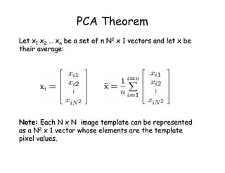
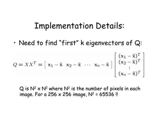
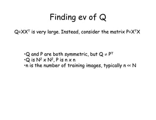
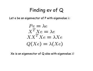
Let Q = X XT be the N2 x N2 matrix:
Notes:
1. Q is square
2. Q is symmetric
3. Q is the covariance matrix [aka scatter matrix]
4. Q can be very large (remember that N2 is the number of
pixels in the template)
20. PCA Theorem
Theorem:
Each xj can be written as:
where ei are the n eigenvectors of Q with non-zero
eigenvalues.
Notes:
1. The eigenvectors e1 e2 … en span an eigenspace
2. e1 e2 … en are N2 x 1 orthonormal vectors (N x N images).
3. The scalars gji are the coordinates of xj in the space.
4.
21. Using PCA to Compress Data
• Expressing x in terms of e1 … en has not
changed the size of the data
• However, if the templates are highly
correlated many of the coordinates of x will be
zero or closed to zero.
note: this means they lie in a
lower-dimensional linear subspace
22. Using PCA to Compress Data
• Sort the eigenvectors ei according to
their eigenvalue:
•Assuming that
•Then
23. Eigenspaces:
Efficient Image Storage
•Use PCA to compress the data:
• each image is stored as a k-
dimensional vector
•Need to store k N x N
eigenvectors
•k << n << N2
a01 a02 a03 a04 a05 a06
24. Eigenspaces:
Efficient Image Comparison
•Use the same procedure to
compress the given image to a k-
dimensional vector.
•Compare the compressed vectors:
•Dot product of k-dimensional vectors
•k << n << N2
a01 a02 a03 a04 a05 a06
25. Implementation Details:
• Need to find “first” k eigenvectors of Q:
Q is N2 x N2 where N2 is the number of pixels in each
image. For a 256 x 256 image, N2 = 65536 !!
26. Finding ev of Q
Q=XXT is very large. Instead, consider the matrix P=XTX
•Q and P are both symmetric, but Q PT
•Q is N2 x N2, P is n x n
•n is the number of training images, typically n << N
27. Finding ev of Q
Let e be an eigenvector of P with eigenvalue :
Xe is an eigenvector of Q also with eigenvalue !
28. Singular Value Decomposition
(SVD)
Any m x n matrix X can be written as the product of 3
matrices:
Where:
• U is m x m and its columns are orthonormal vectors
• V is n x n and its columns are orthonormal vectors
• D is m x n diagonal and its diagonal elements are called
the singular values of X, and are such that:
1 ¸ 2 ¸ … n ¸ 0
29. SVD Properties
• The columns of U are the eigenvectors of XXT
• The columns of V are the eigenvectors of XTX
• The squares of the diagonal elements of D are the
eigenvalues of XXT and XTX
30. Algorithm EIGENSPACE_LEARN
Assumptions:
1. Each image contains one object only.
2. Objects are imaged by a fixed camera .
3. Images are normalized in size N x N:
• The image frame is the minimum rectangle enclosing the object.
4. Energy of pixels values is normalized to 1:
• ij I(i,j)2 = 1
5. The object is completely visible and
unoccluded in all images.
31. Algorithm EIGENSPACE_LEARN
Getting the data:
For each object o to be represented, o = 1, …,O
1. Place o on a turntable, acquire a set of n images
by rotating the table in increments of 360o/n
2. For each image p, p = 1, …, n:
1. Segment o from the background
2. Normalize the image size and energy
3. Arrange the pixels as vectors xop
32. Algorithm EIGENSPACE_LEARN
Storing the data:
1. Find the average image vector
2. Assemble the matrix X:
3. Find the first k eigenvectors of XXT: e1,…,ek
(use XTX or SVD)
4. For each object o, each image p:
•Compute the corresponding k-dimensional point:
33. Algorithm EIGENSPACE_IDENTIF
Recognizing an object from the DB:
1. Given an image, segment the object from the background
2. Normalize the size an energy, write it as a vector i
3. Compute the corresponding k-dimensional point:
4. Find the closest gop k-dimensional point to g
34. Key Property of Eigenspace Representation
Given
• 2 images ˆ ˆ
x1 , x2 that are used to construct the Eigenspace
• ˆ ˆ
g1 is the eigenspace projection of image x1
• ˆ ˆ
g 2 is the eigenspace projection of image x2
Then,
|| g 2 g1 || || x2 x1 ||
ˆ ˆ ˆ ˆ
That is, distance in Eigenspace is approximately equal to the
correlation between two images.
35. Example: Murase and Nayar, 1996
Database of
objects. No
background
clutter or
occlusion
36. Murase and Nayar, 1996
• Acquire models of object appearances
using a turntable
37.
38.
39. Example: EigenFaces
These slides from S. Narasimhan, CMU
= +
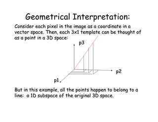
• An image is a point in a high dimensional space
– An N x M image is a point in RNM
– We can define vectors in this space as we did in the 2D case
[Thanks to Chuck Dyer, Steve Seitz, Nishino]
40. Dimensionality Reduction
The set of faces is a “subspace” of the
set
of images
– Suppose it is K dimensional
– We can find the best subspace using
PCA
– This is like fitting a “hyper-plane” to
the set of faces
• spanned by vectors v1, v2, ..., vK
Any face:
41. Generating Eigenfaces – in words
1. Large set of images of human faces is taken.
2. The images are normalized to line up the
eyes, mouths and other features.
3. The eigenvectors of the covariance matrix
of the face image vectors are then
extracted.
4. These eigenvectors are called eigenfaces.
42. Eigenfaces
“mean” face
Eigenfaces look somewhat like generic faces.
43. Eigenfaces for Face Recognition
• When properly weighted, eigenfaces can be
summed together to create an approximate
gray-scale rendering of a human face.
• Remarkably few eigenvector terms are needed
to give a fair likeness of most people's faces.
• Hence eigenfaces provide a means of applying
data compression to faces for identification
purposes.
44. Eigenfaces
• PCA extracts the eigenvectors of A
– Gives a set of vectors v1, v2, v3, ...
– Each one of these vectors is a direction in face space
• what do these look like?
45. Projecting onto the Eigenfaces
• The eigenfaces v1, ..., vK span the space of
faces
– A face is converted to eigenface coordinates by
47. Recognition with Eigenfaces
• Algorithm
1. Process the image database (set of images with labels)
• Run PCA—compute eigenfaces
• Calculate the K coefficients for each image
2. Given a new image (to be recognized) x, calculate K
coefficients
3. Detect if x is a face
4. If it is a face, who is it?
• Find closest labeled face in database
• nearest-neighbor in K-dimensional space
48. Cautionary Note:
PCA has problems with occlusion
p2 because it uses global information
e2
e1
a1 a0
p1
and also, more generally, with outliers
PCA