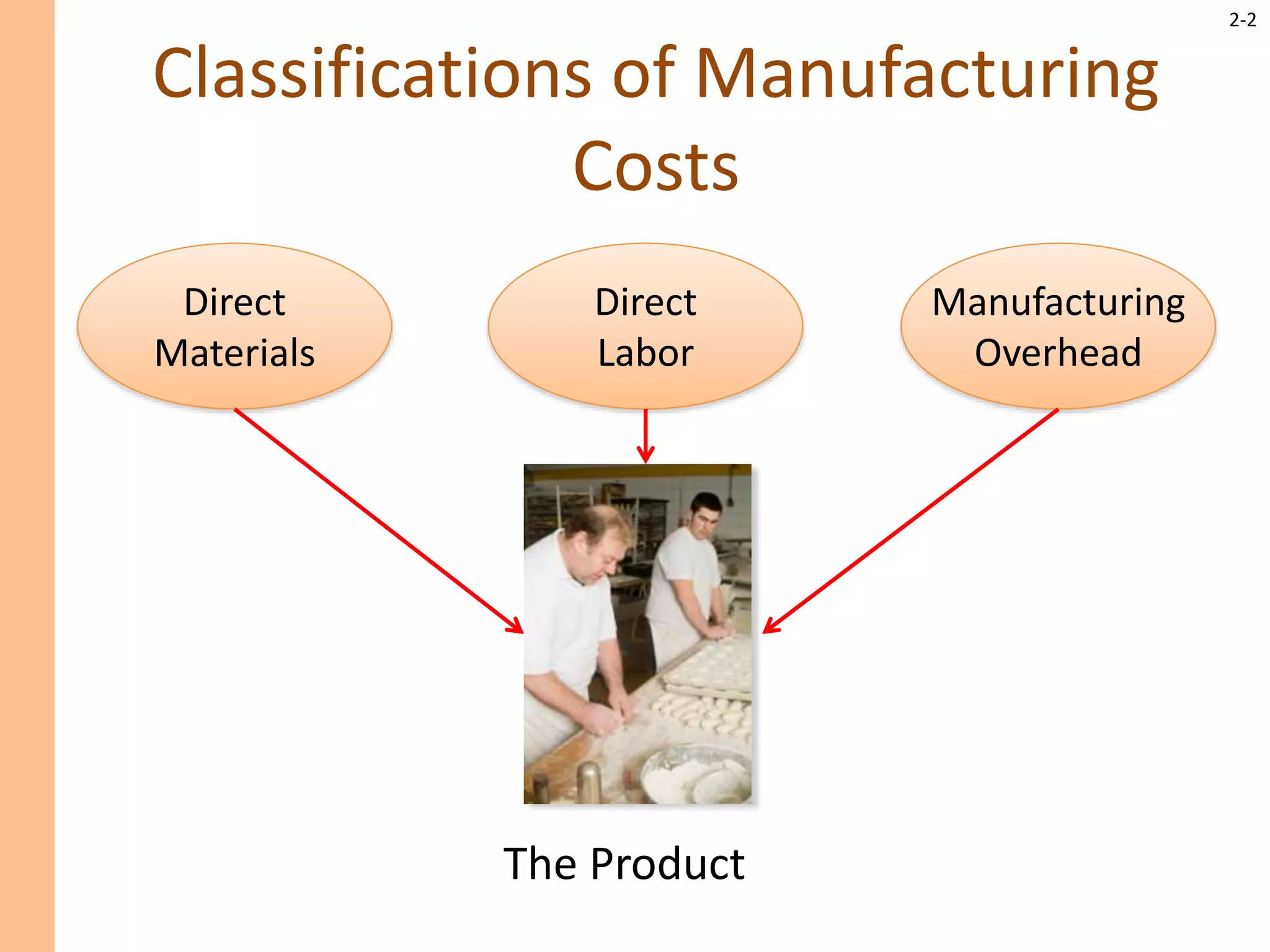
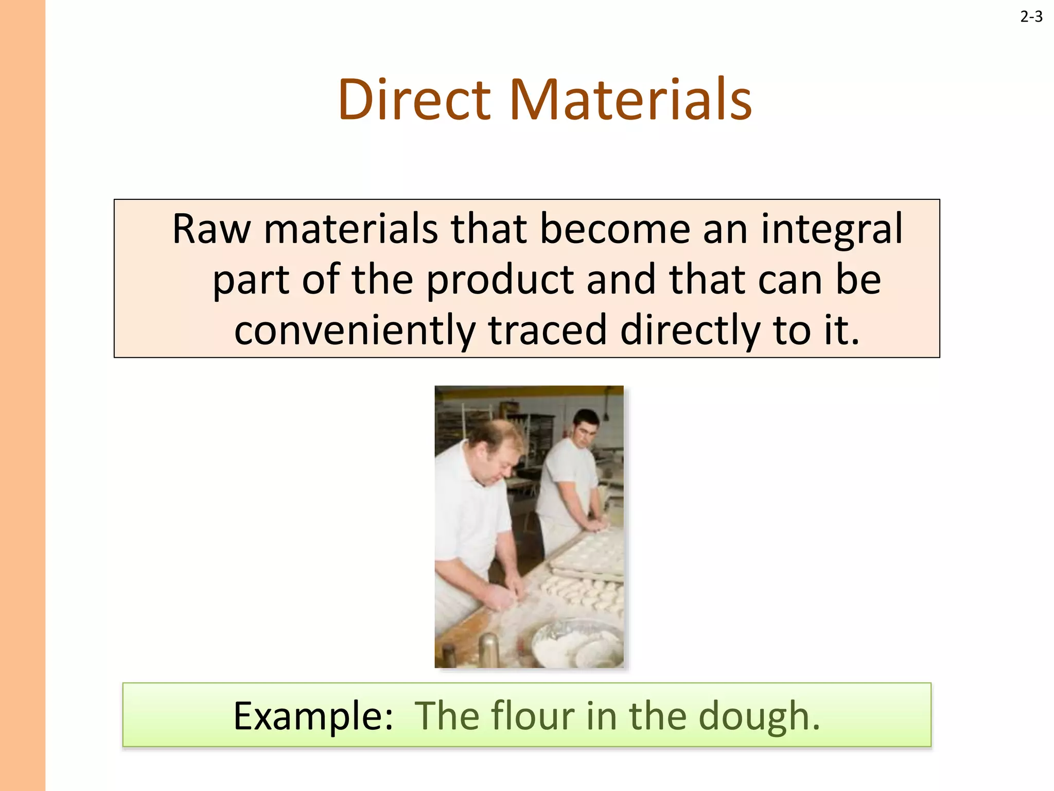
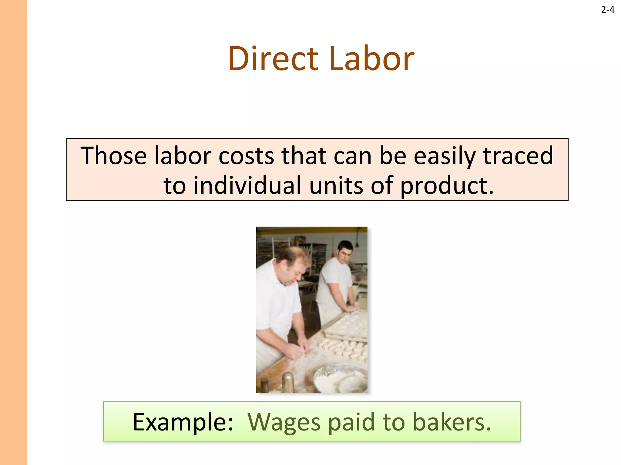
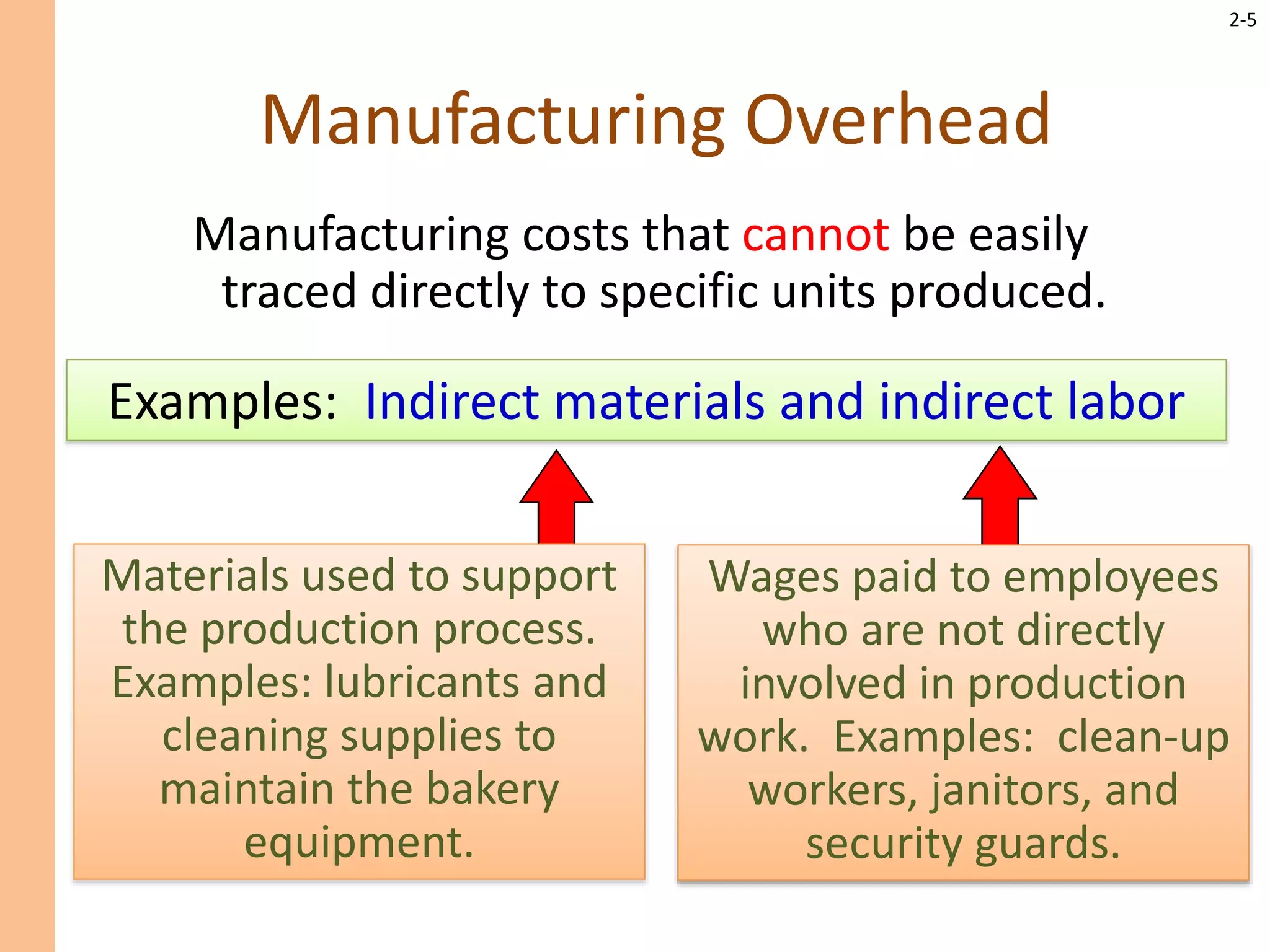
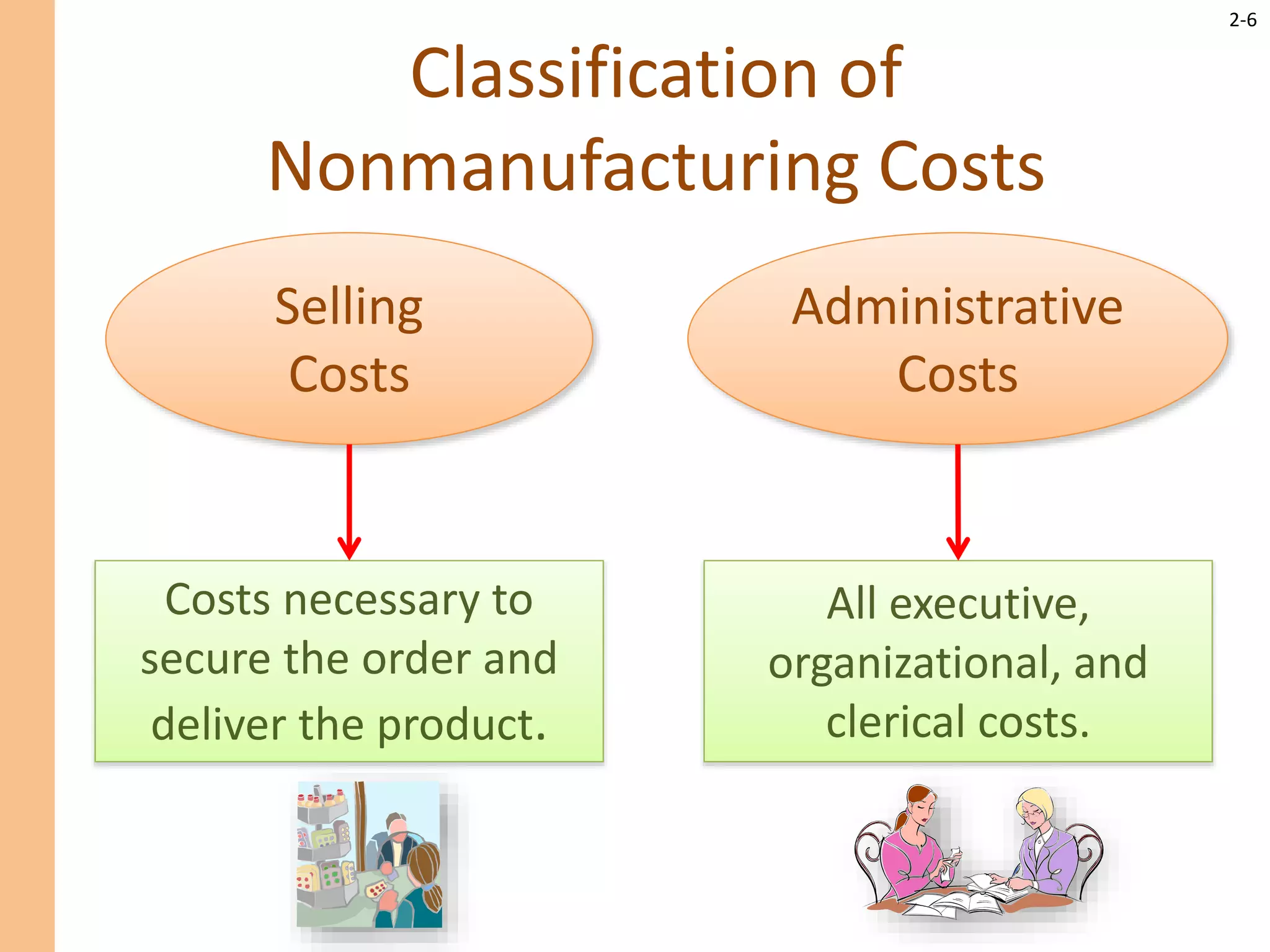
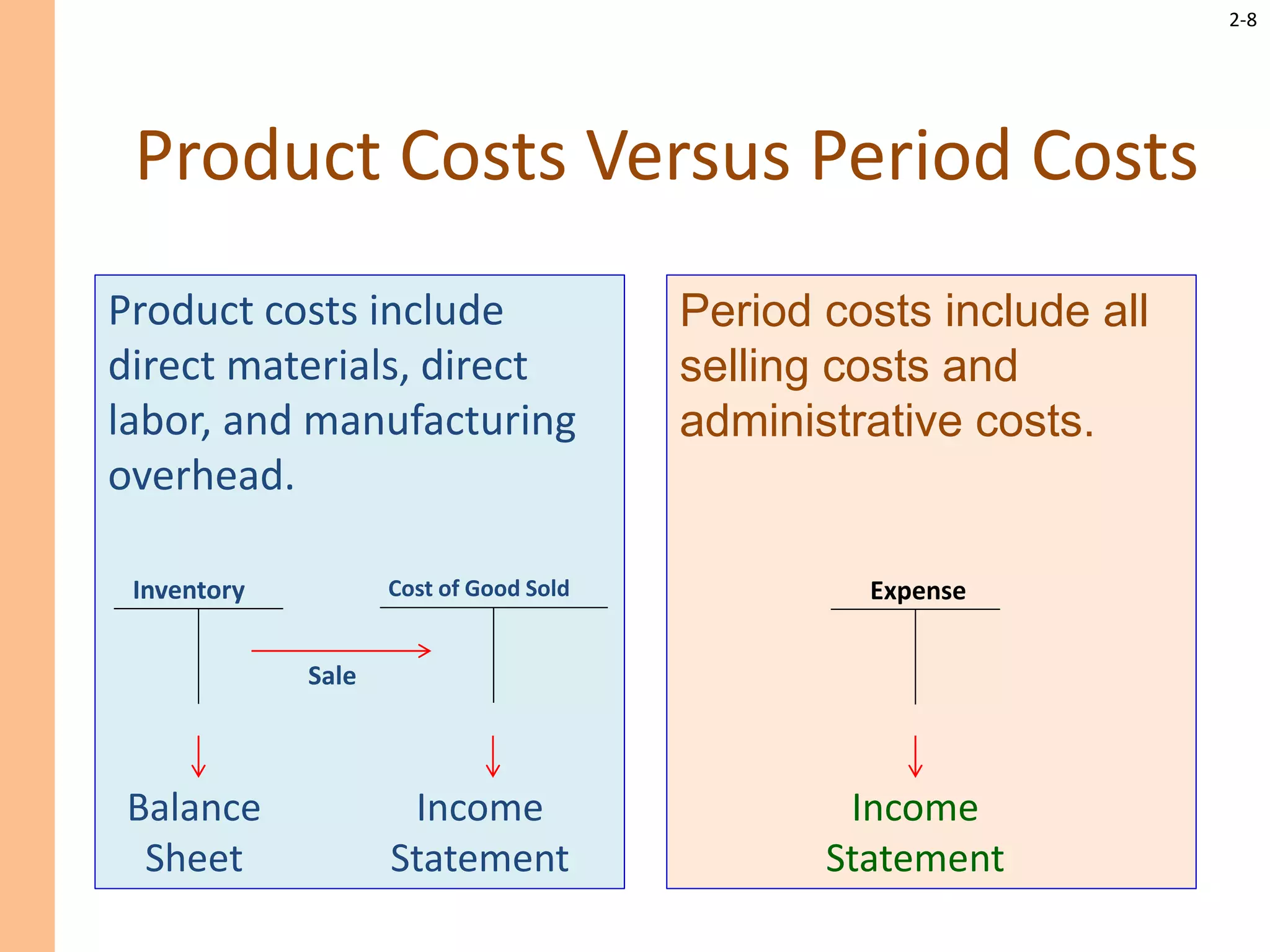
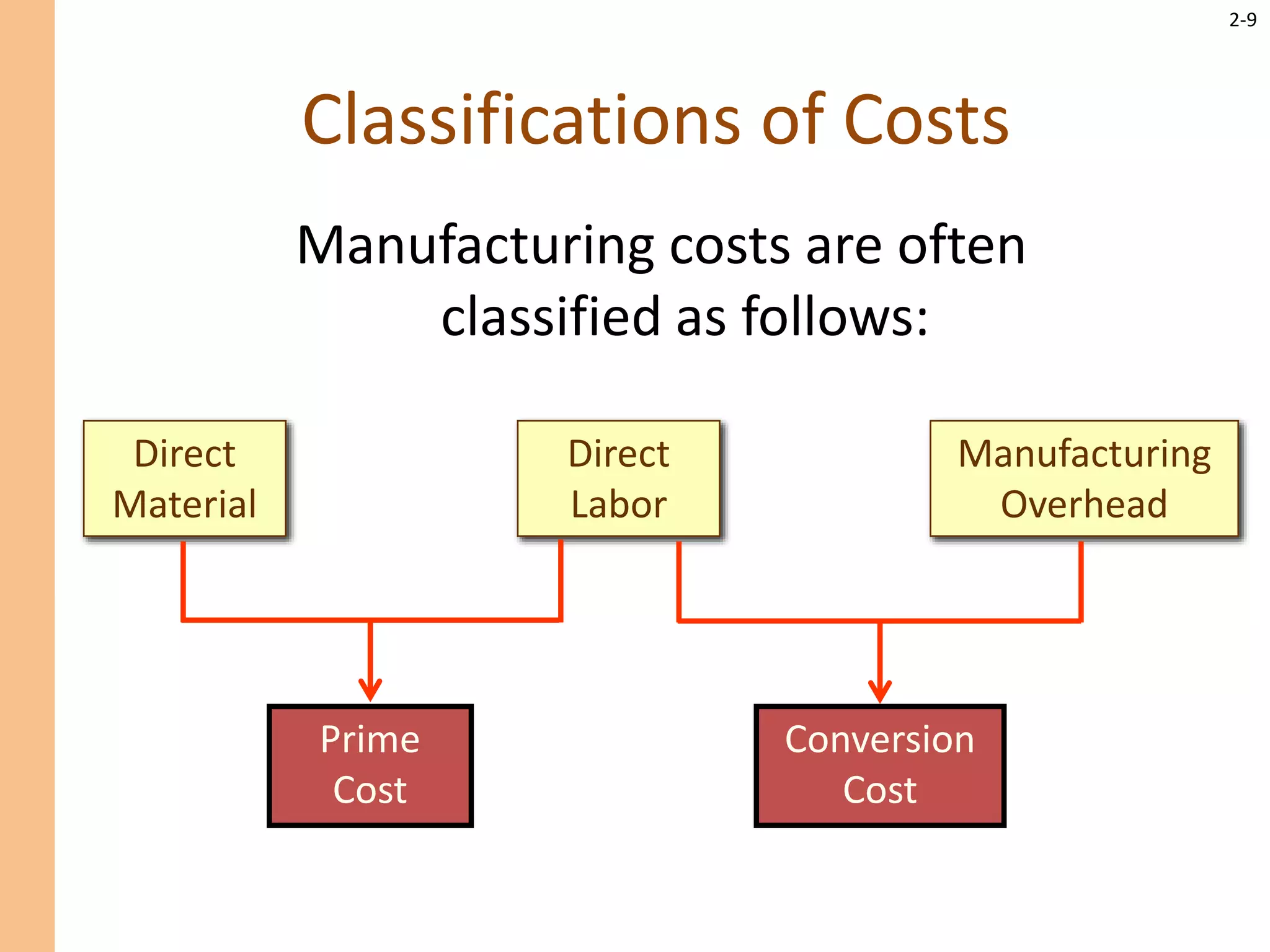
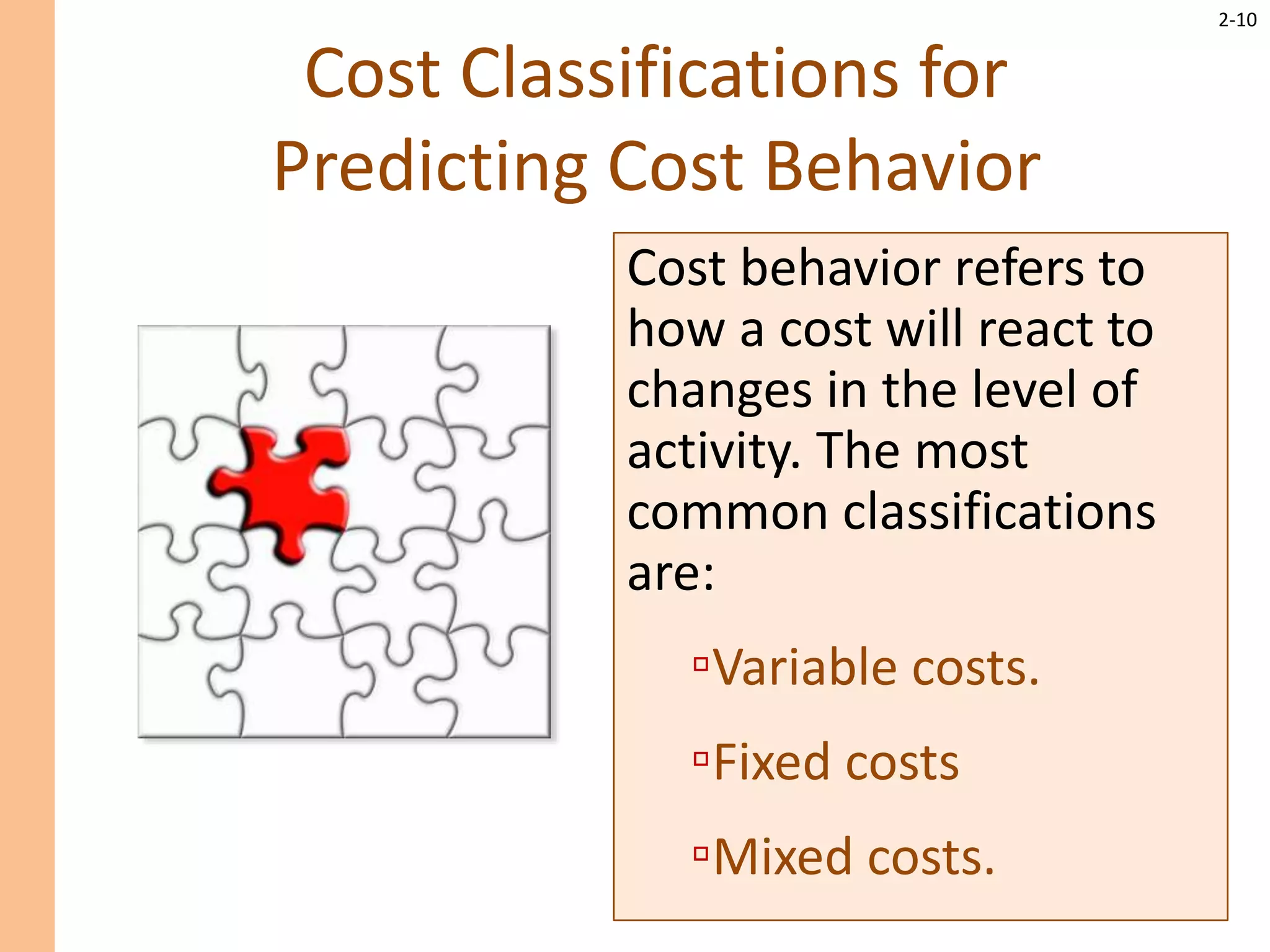
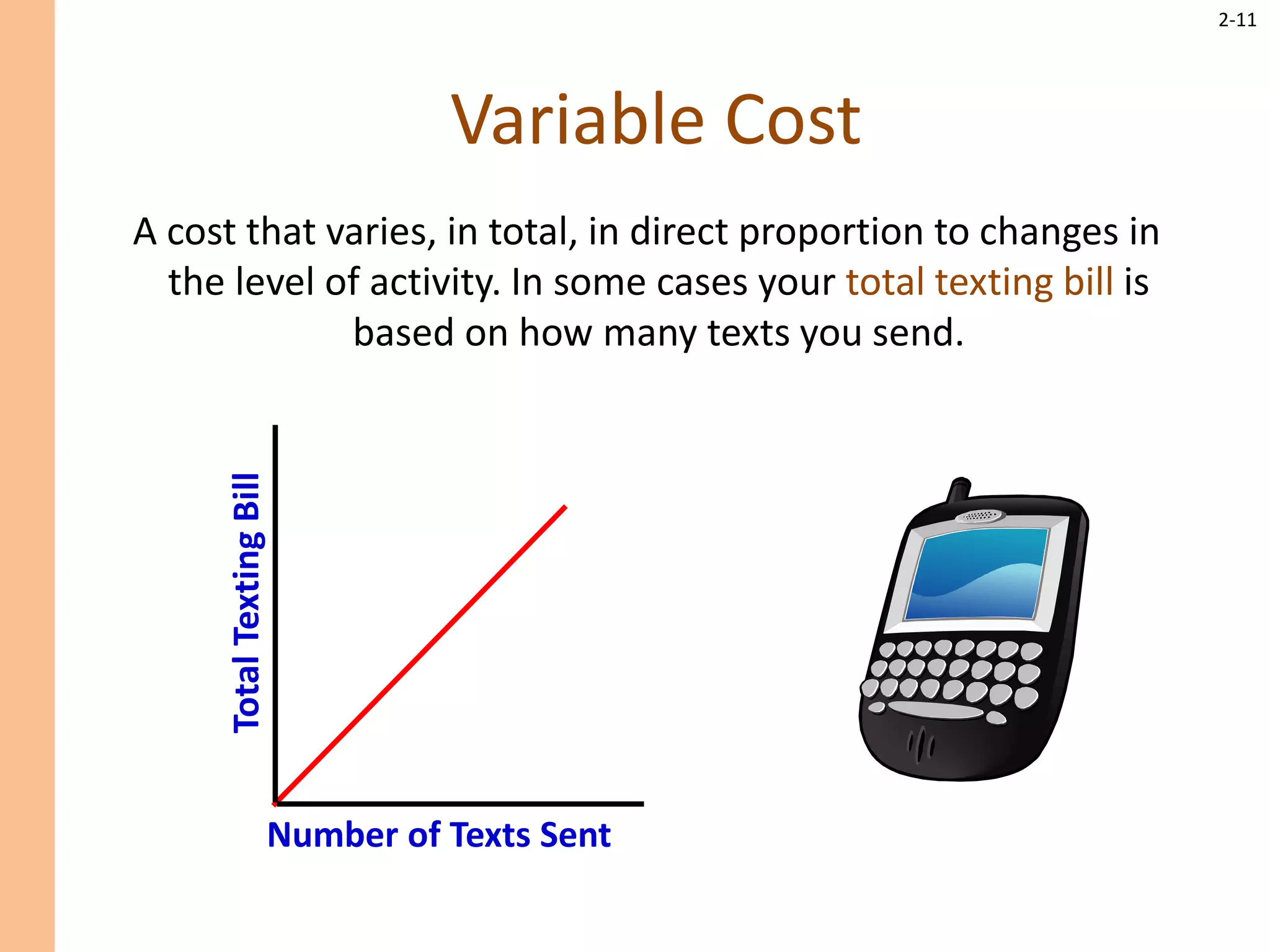
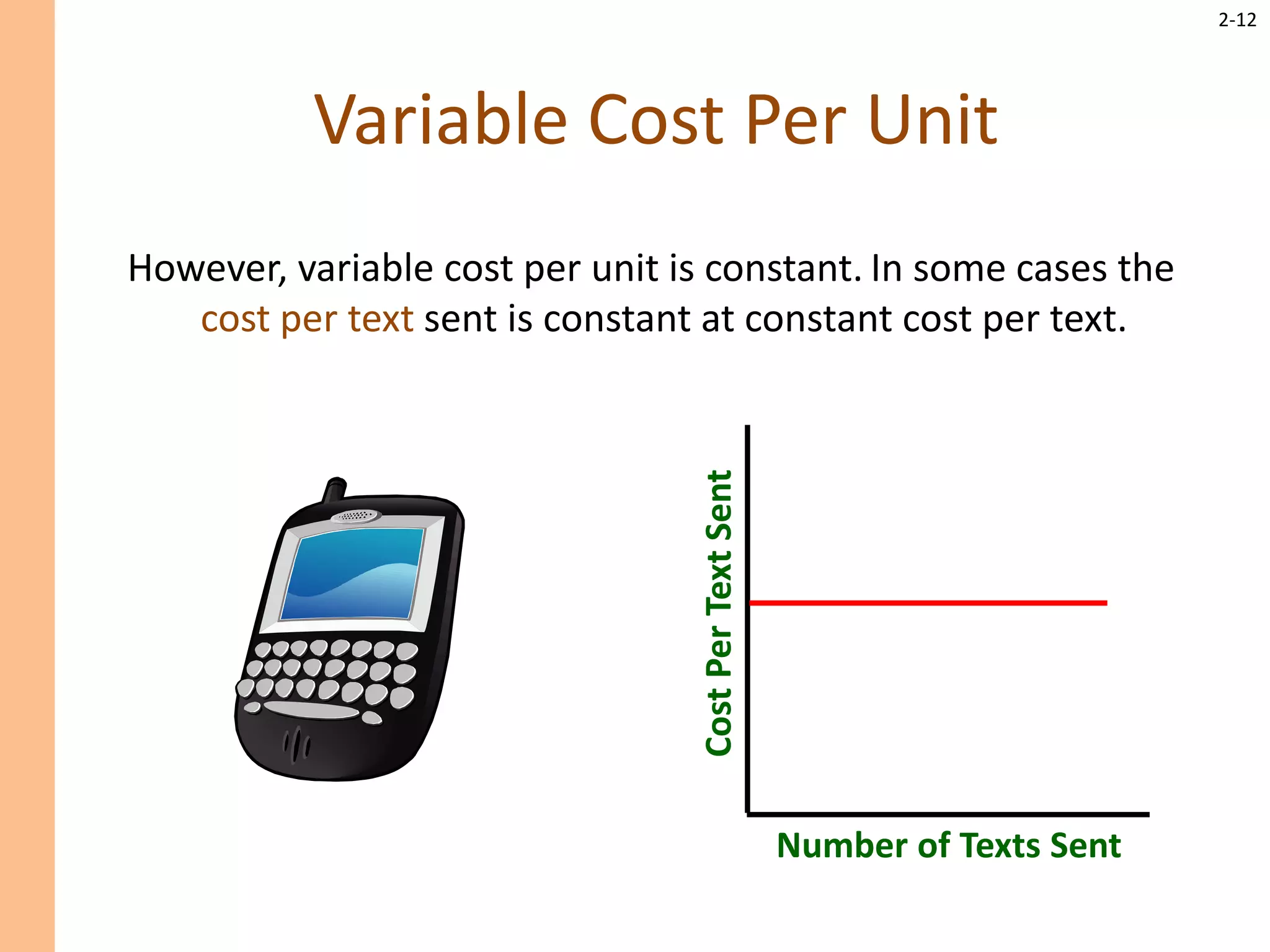
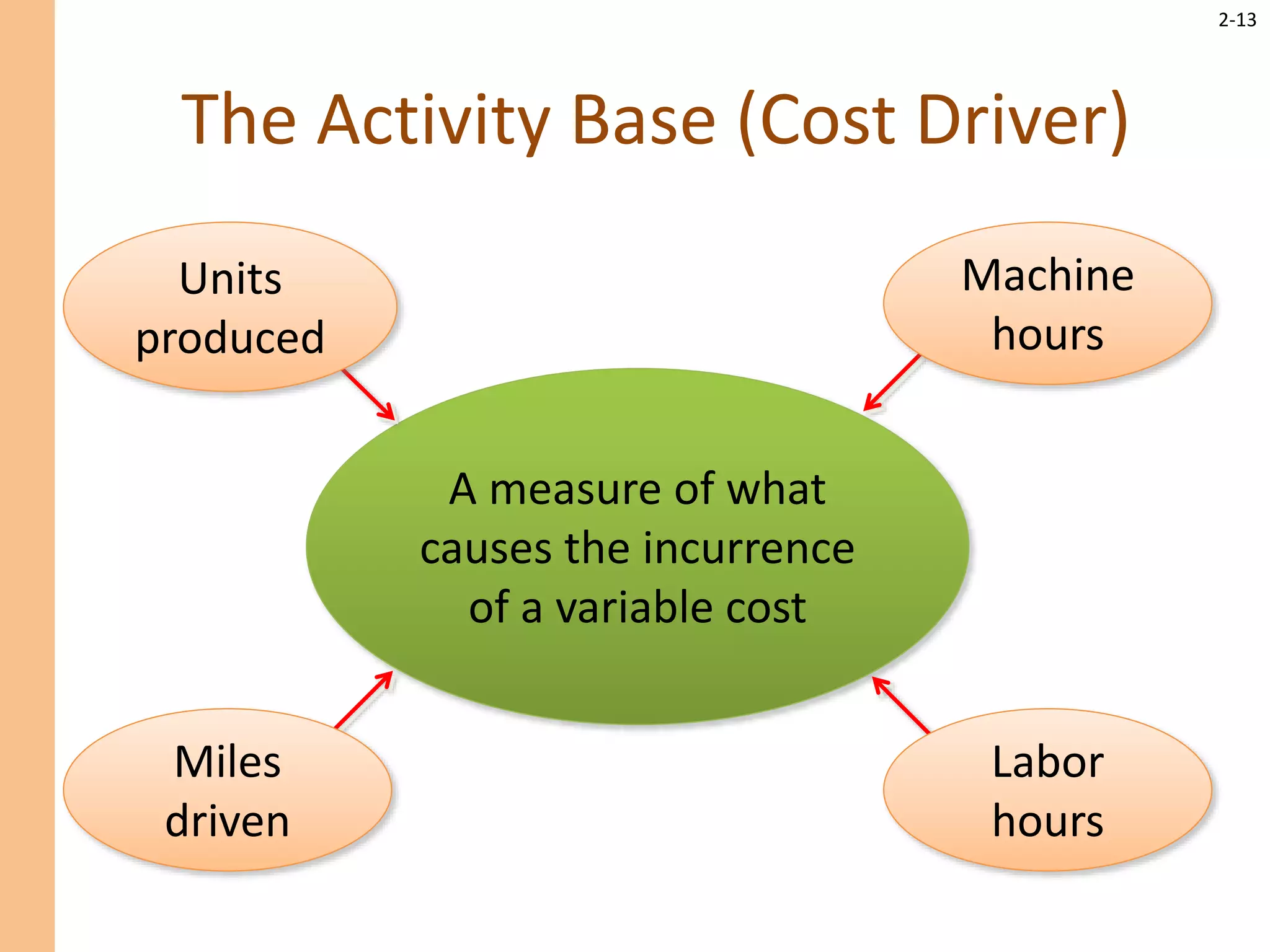
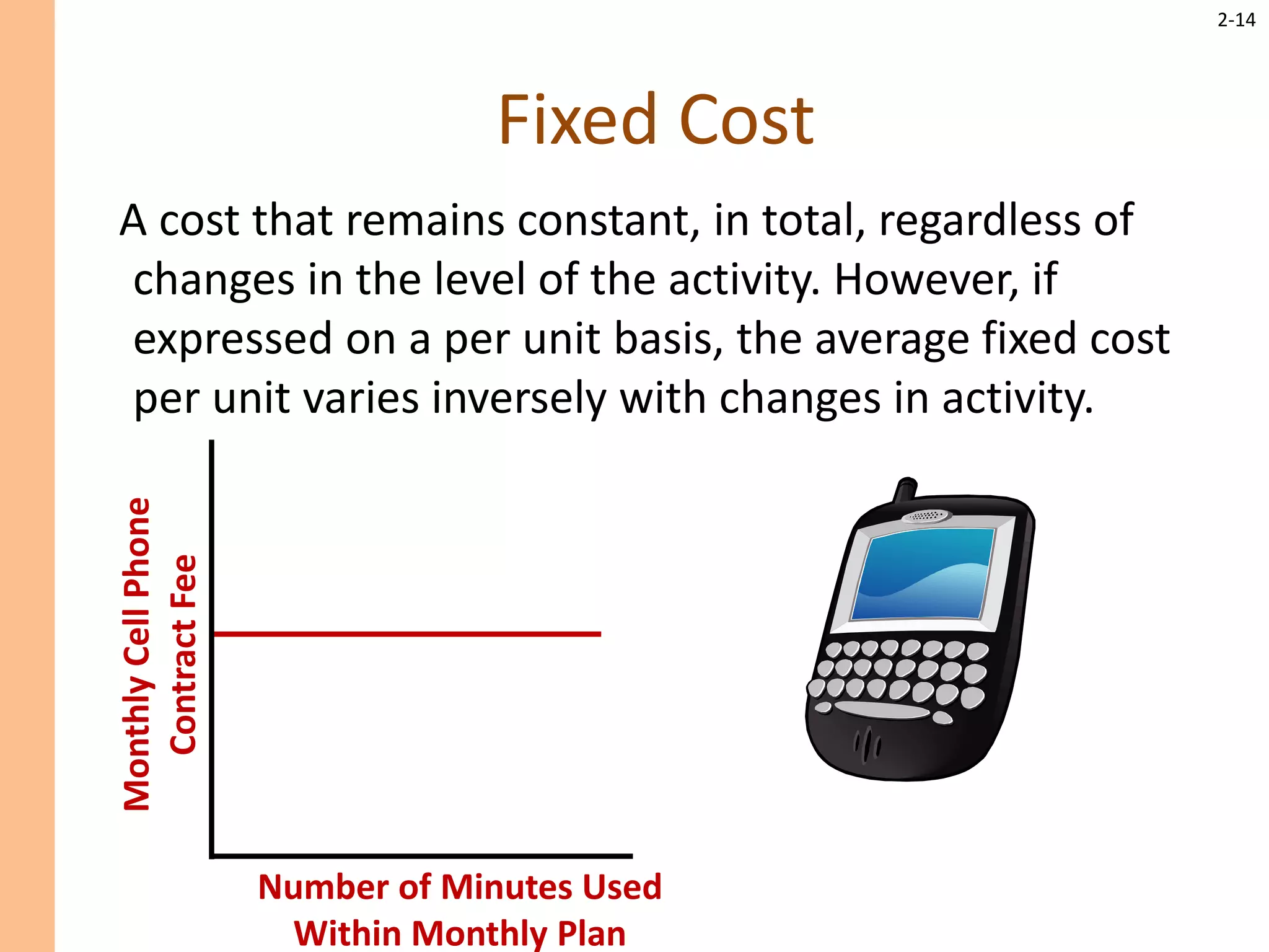
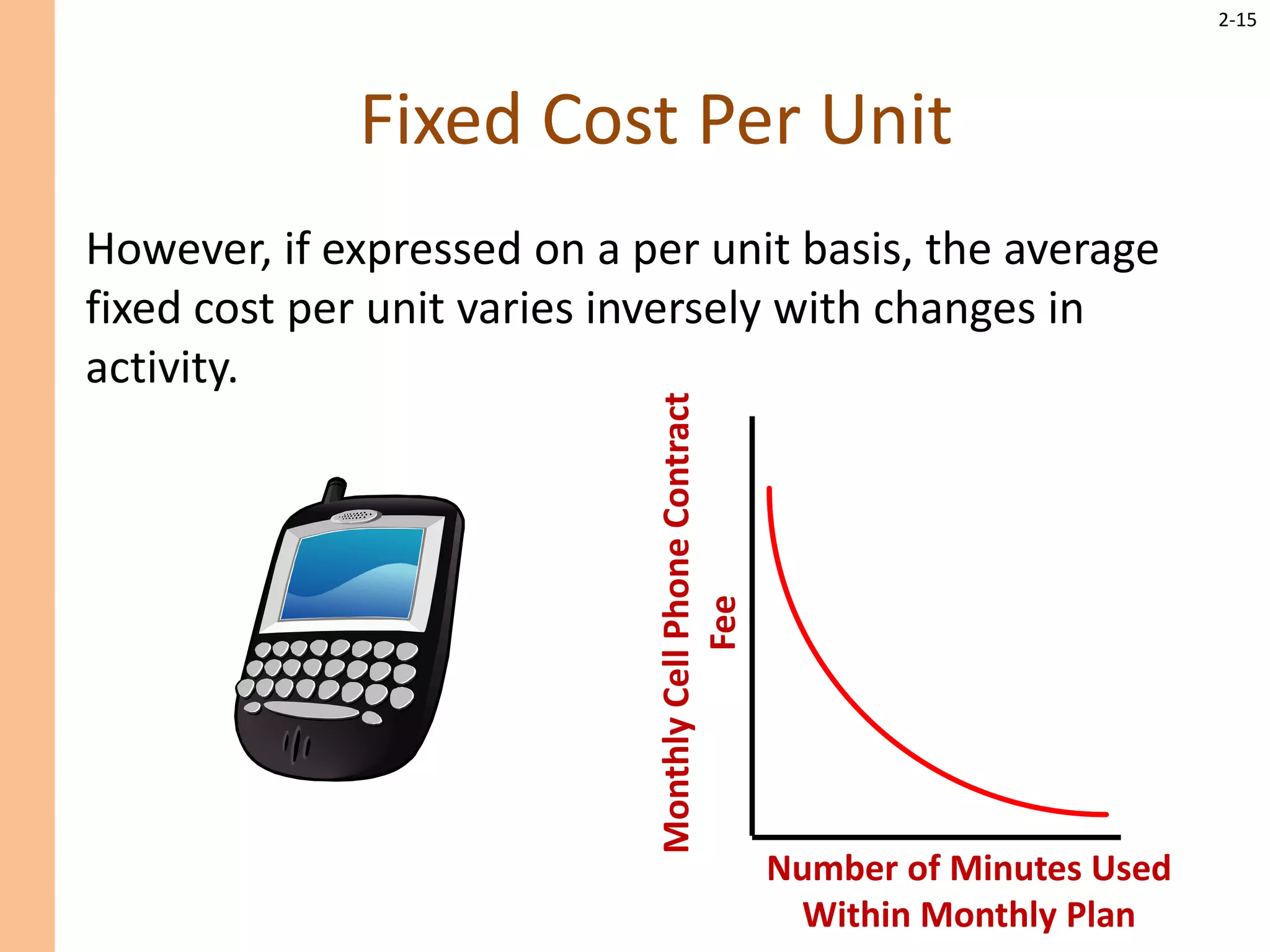
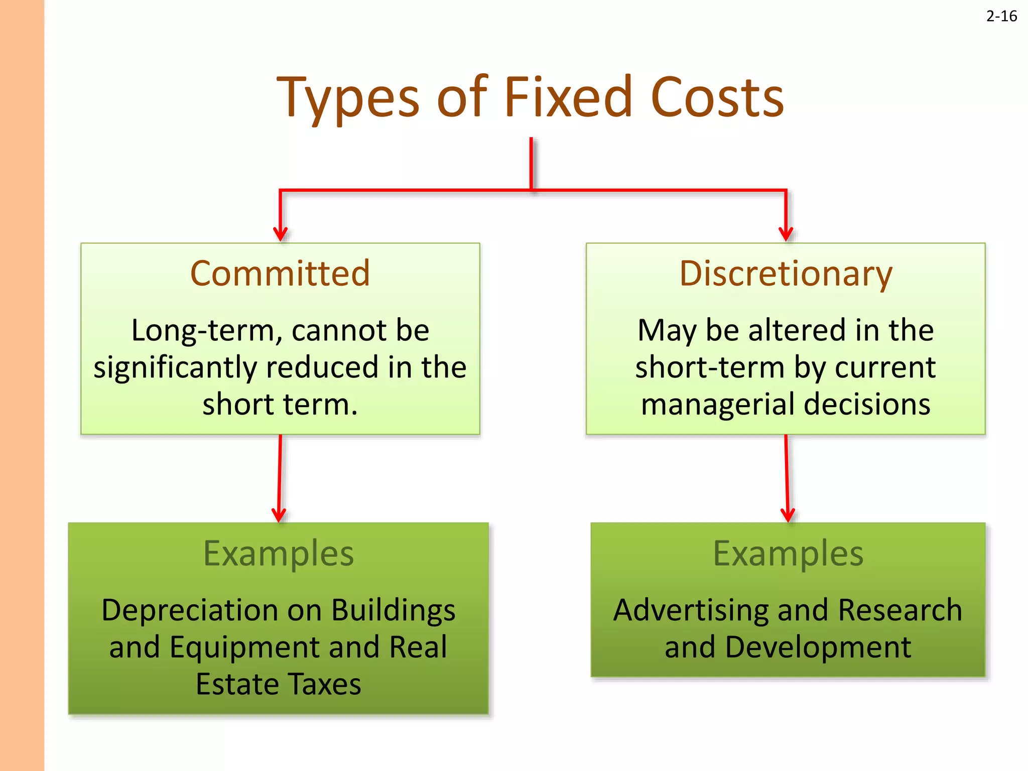
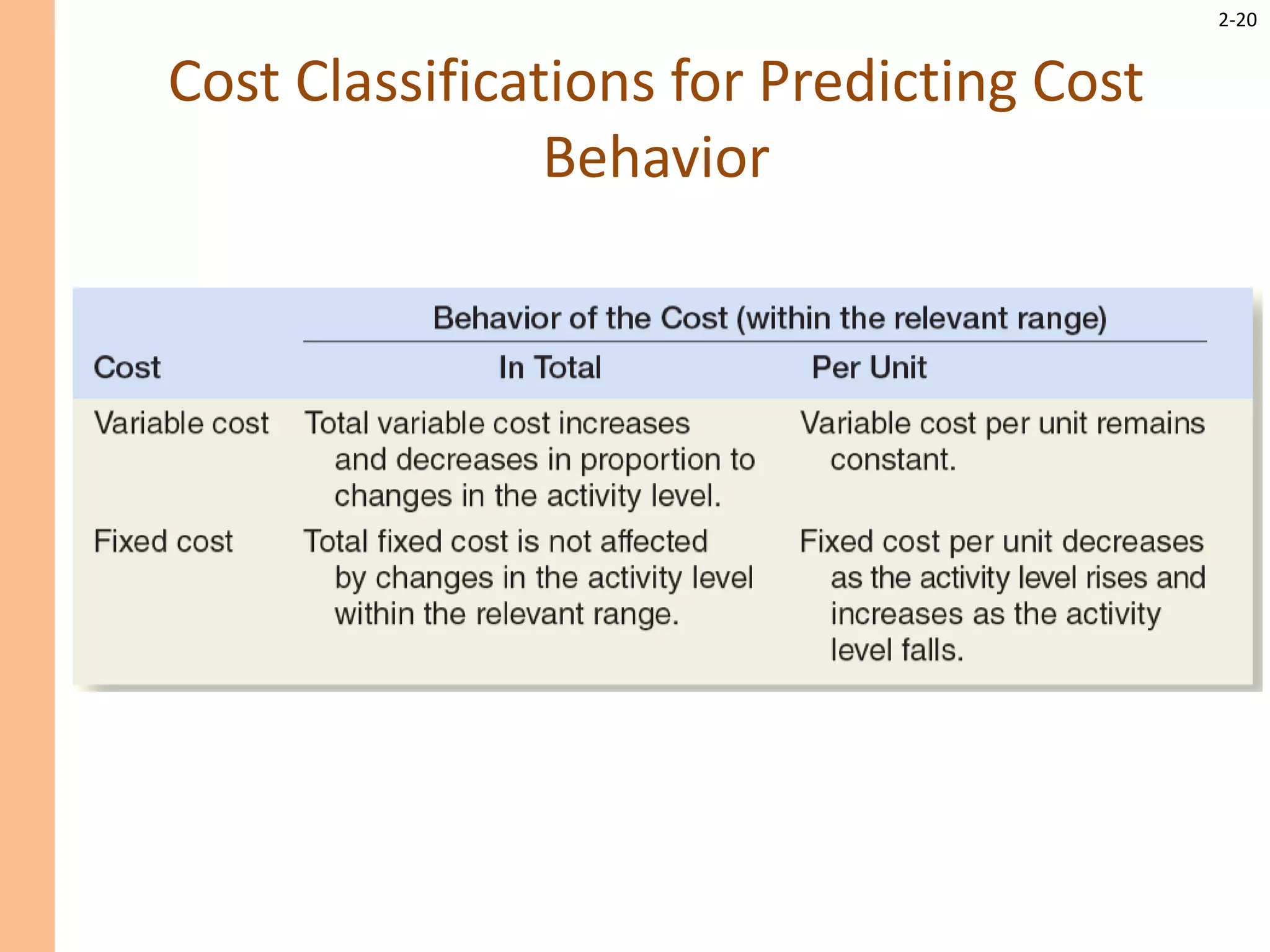
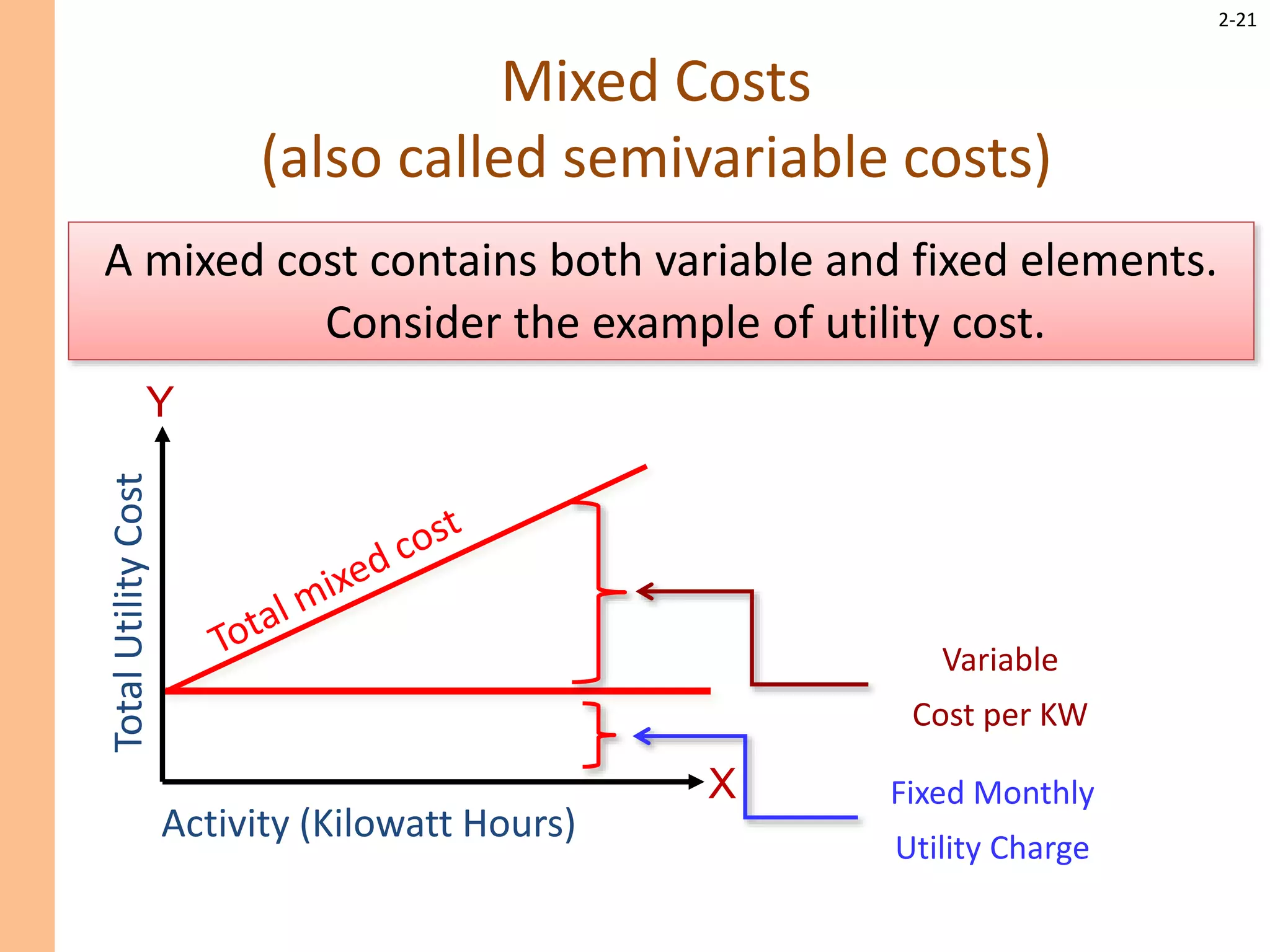
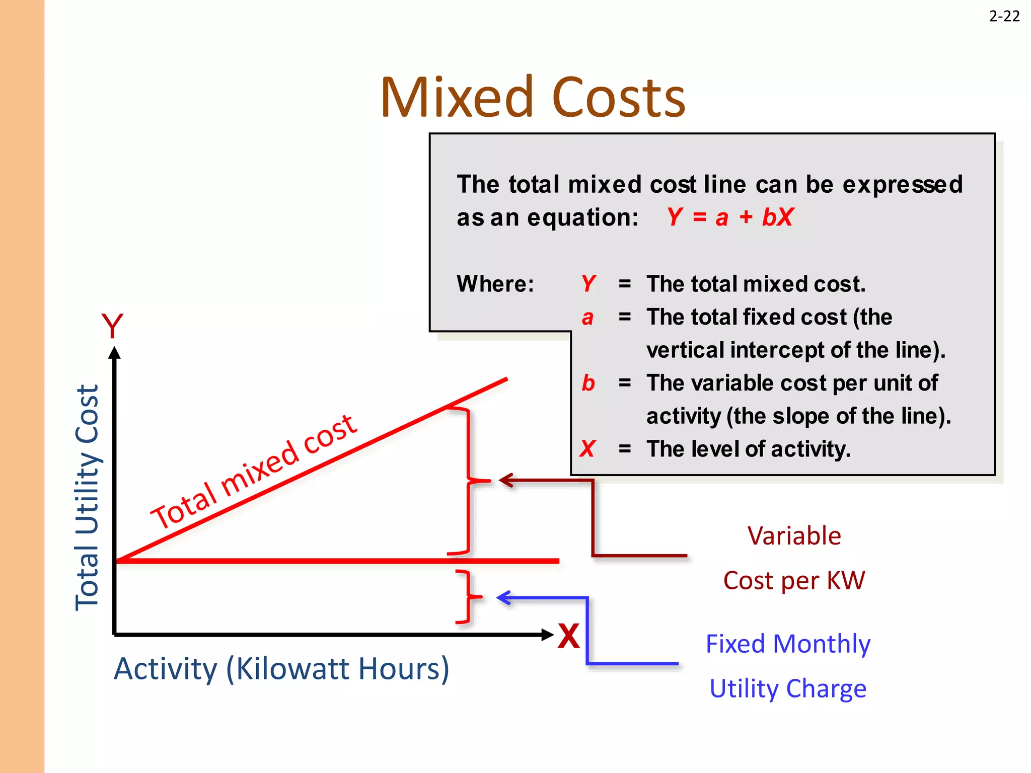
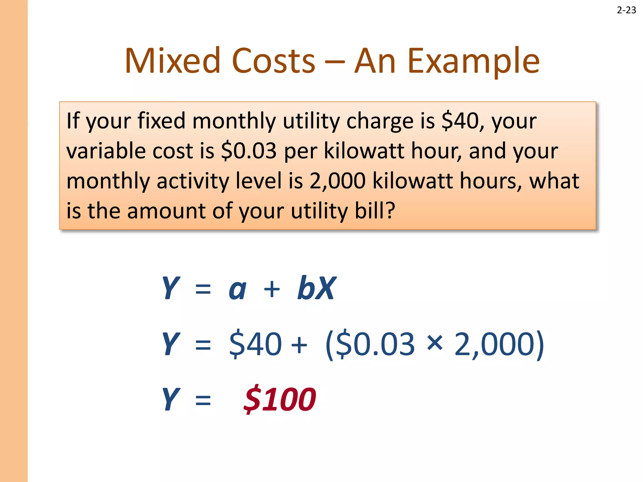
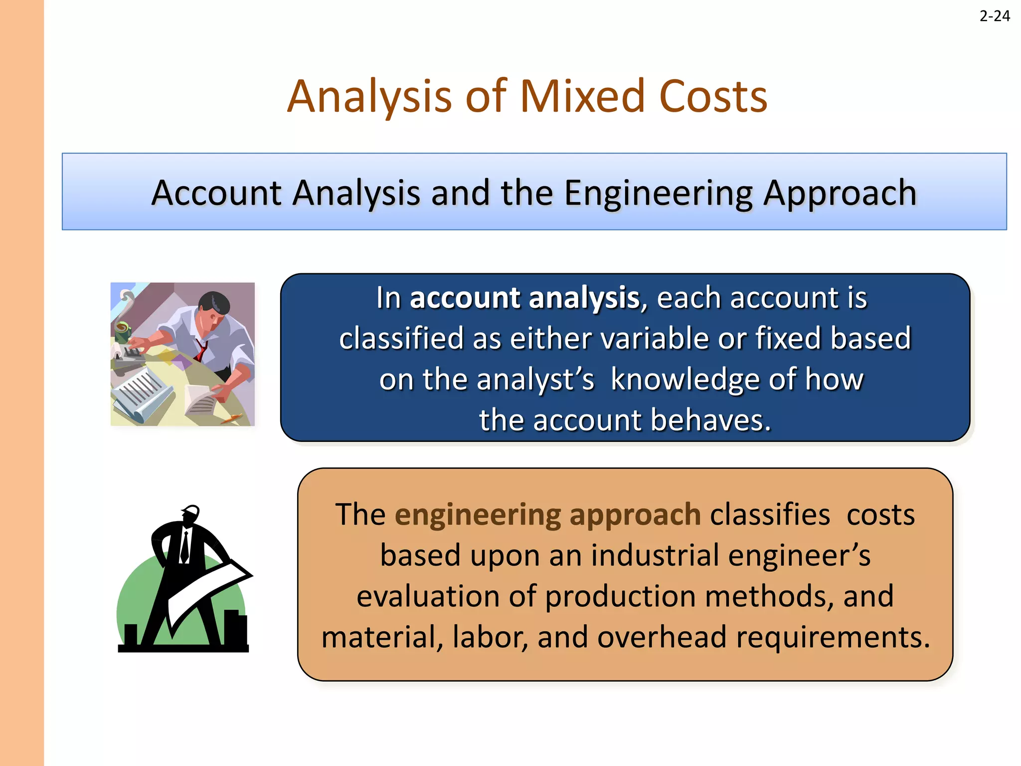
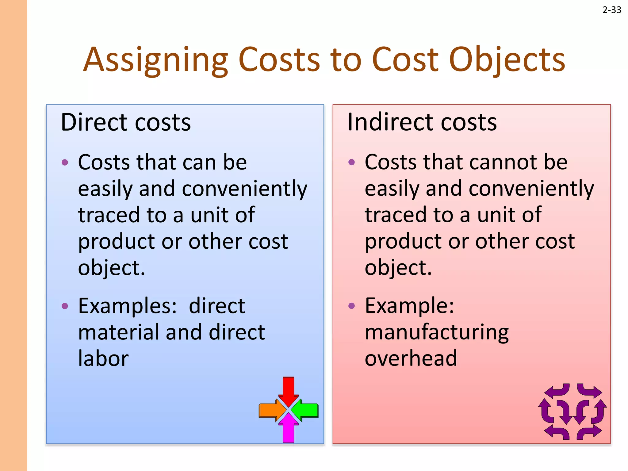
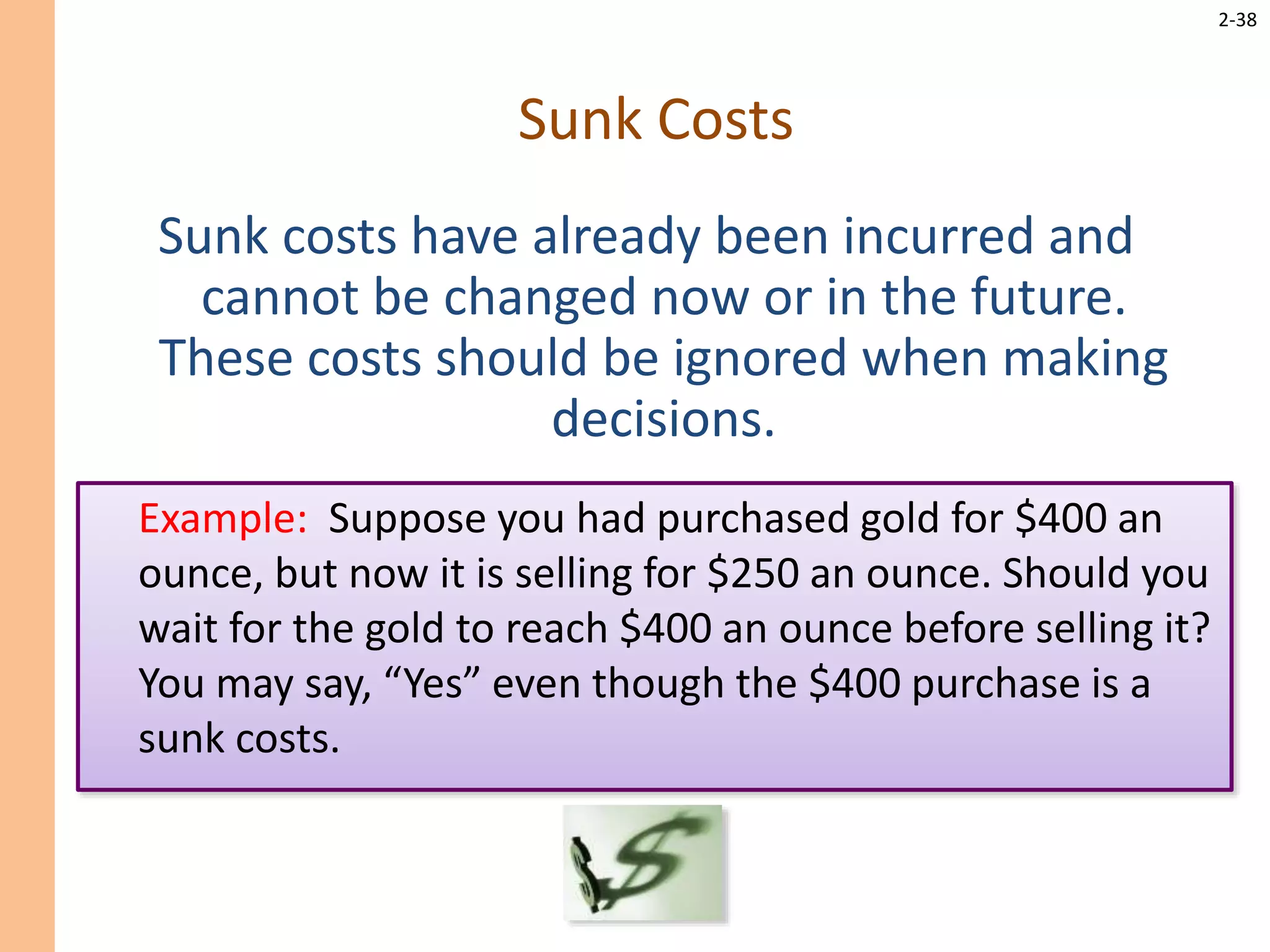
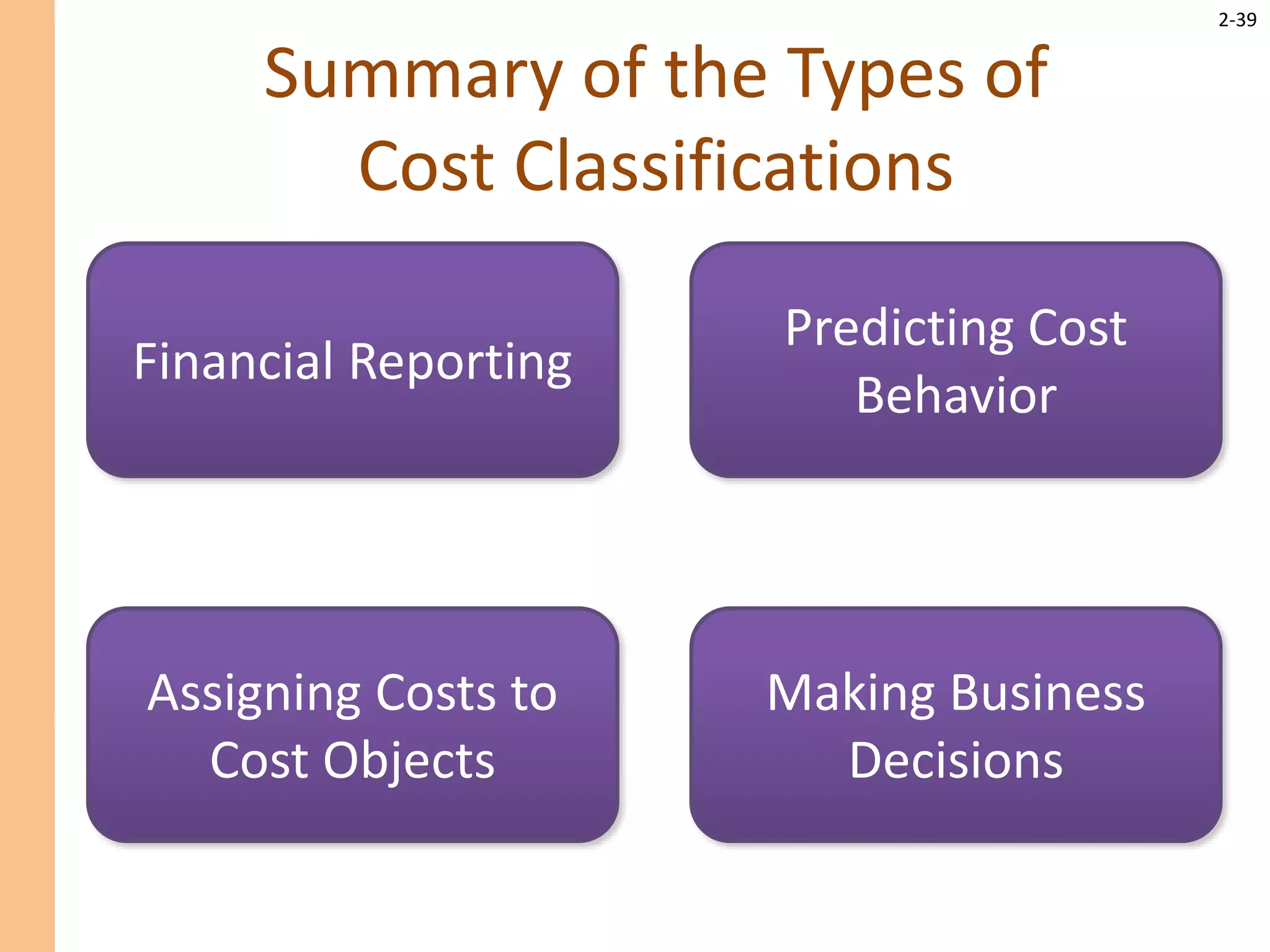
This document provides an overview of different classifications of costs that are important for managerial accounting. It discusses direct materials, direct labor, and manufacturing overhead as the three main classifications of manufacturing costs. It also defines product costs, which become part of inventory, and period costs, which are expensed immediately. Additionally, it examines classifications of costs based on their behavior when activity changes, including variable, fixed, and mixed costs. Differential costs, opportunity costs, and sunk costs are identified as important classifications for decision making.

1. PowerPoint Authors:
Susan Coomer Galbreath, Ph.D., CPA
Charles W. Caldwell, D.B.A., CMA
Jon A. Booker, Ph.D., CPA, CIA
Cynthia J. Rooney, Ph.D., CPA
Copyright © 2014 by The McGraw-Hill Companies, Inc. All rights reserved.
Managerial Accounting and Cost
Concepts
Chapter 2

2. 2-2
The Product
Classifications of Manufacturing
Costs
Direct
Materials
Manufacturing
Overhead
Direct
Labor

3. 2-3
Direct Materials
Raw materials that become an integral
part of the product and that can be
conveniently traced directly to it.
Example: The flour in the dough.

4. 2-4
Direct Labor
Those labor costs that can be easily traced
to individual units of product.
Example: Wages paid to bakers.

5. 2-5
Manufacturing Overhead
Manufacturing costs that cannot be easily
traced directly to specific units produced.
Examples: Indirect materials and indirect labor
Wages paid to employees
who are not directly
involved in production
work. Examples: clean-up
workers, janitors, and
security guards.
Materials used to support
the production process.
Examples: lubricants and
cleaning supplies to
maintain the bakery
equipment.

6. 2-6
Classification of
Nonmanufacturing Costs
Selling
Costs
Costs necessary to
secure the order and
deliver the product.
Administrative
Costs
All executive,
organizational, and
clerical costs.

7. 2-7
Product costs and period costs

8. 2-8
Product Costs Versus Period Costs
Product costs include
direct materials, direct
labor, and manufacturing
overhead.
Period costs include all
selling costs and
administrative costs.
Inventory Cost of Good Sold
Balance
Sheet
Income
Statement
Sale
Expense
Income
Statement

9. 2-9
Classifications of Costs
Manufacturing costs are often
classified as follows:
Direct
Material
Direct
Labor
Manufacturing
Overhead
Prime
Cost
Conversion
Cost

10. 2-10
Cost Classifications for
Predicting Cost Behavior
Cost behavior refers to
how a cost will react to
changes in the level of
activity. The most
common classifications
are:
▫Variable costs.
▫Fixed costs
▫Mixed costs.

11. 2-11
Variable Cost
A cost that varies, in total, in direct proportion to changes in
the level of activity. In some cases your total texting bill is
based on how many texts you send.
Number of Texts Sent
Total
Texting
Bill

12. 2-12
Variable Cost Per Unit
However, variable cost per unit is constant. In some cases the
cost per text sent is constant at constant cost per text.
Number of Texts Sent
Cost
Per
Text
Sent

13. 2-13
The Activity Base (Cost Driver)
A measure of what
causes the incurrence
of a variable cost
Labor
hours
Units
produced
Machine
hours
Miles
driven

14. 2-14
Fixed Cost
A cost that remains constant, in total, regardless of
changes in the level of the activity. However, if
expressed on a per unit basis, the average fixed cost
per unit varies inversely with changes in activity.
Number of Minutes Used
Within Monthly Plan
Monthly
Cell
Phone
Contract
Fee

15. 2-15
Fixed Cost Per Unit
However, if expressed on a per unit basis, the average
fixed cost per unit varies inversely with changes in
activity.
Number of Minutes Used
Within Monthly Plan
Monthly
Cell
Phone
Contract
Fee

16. 2-16
Examples
Advertising and Research
and Development
Examples
Depreciation on Buildings
and Equipment and Real
Estate Taxes
Types of Fixed Costs
Discretionary
May be altered in the
short-term by current
managerial decisions
Committed
Long-term, cannot be
significantly reduced in the
short term.

17. 2-17
A straight line
closely
approximates a
curvilinear
variable cost line
within the
relevant range.
The Linearity Assumption and
the Relevant Range

18. 2-18
Fixed Costs and the Relevant Range
Fixed costs would increase in a
step fashion at a rate of
$30,000 for each additional
1,000 square feet.
For example, assume office space is available at a
rental rate of $30,000 per year in increments of
1,000 square feet.

19. 2-19
Rent
Cost
in
Thousands
of
Dollars
0 1,000 2,000 3,000
Rented Area (Square Feet)
0
30
60
Fixed Costs and the Relevant Range
90
Relevant
Range
The relevant range
of activity for a fixed
cost is the range of
activity over which
the graph of the
cost is flat.

20. 2-20
Cost Classifications for Predicting Cost
Behavior

21. 2-21
Fixed Monthly
Utility Charge
Variable
Cost per KW
Activity (Kilowatt Hours)
Total
Utility
Cost
X
Y
A mixed cost contains both variable and fixed elements.
Consider the example of utility cost.
Mixed Costs
(also called semivariable costs)

22. 2-22
Mixed Costs
The total mixed cost line can be expressed
as an equation: Y = a + bX
Where: Y = The total mixed cost.
a = The total fixed cost (the
vertical intercept of the line).
b = The variable cost per unit of
activity (the slope of the line).
X = The level of activity.
Fixed Monthly
Utility Charge
Variable
Cost per KW
Activity (Kilowatt Hours)
Total
Utility
Cost
X
Y

23. 2-23
Mixed Costs – An Example
If your fixed monthly utility charge is $40, your
variable cost is $0.03 per kilowatt hour, and your
monthly activity level is 2,000 kilowatt hours, what
is the amount of your utility bill?
Y = a + bX
Y = $40 + ($0.03 × 2,000)
Y = $100

24. 2-24
Analysis of Mixed Costs
In account analysis, each account is
classified as either variable or fixed based
on the analyst’s knowledge of how
the account behaves.
The engineering approach classifies costs
based upon an industrial engineer’s
evaluation of production methods, and
material, labor, and overhead requirements.
Account Analysis and the Engineering Approach

25. 2-25
Scattergraph Plots – An Example
Assume the following hours of maintenance work
and the total maintenance costs for six months.

26. 2-26
Plot the data points on a graph
(Total Cost Y vs. Activity X).
The Scattergraph Method
$7,000
$7,500
$8,000
$8,500
$9,000
$9,500
$10,000
400 500 600 700 800 900
Scattergraph Method
X
Y
Hours of Maintenance
Total
Maintenance
Cost

27. 2-27
The High-Low Method – An
Example
= $6.00/hour
$2,400
400

28. 2-28
The High-Low Method – An
Example
Total Fixed Cost = Total Cost – Total Variable Cost
Total Fixed Cost = $9,800 – ($6/hour × 850 hours)
Total Fixed Cost = $9,800 – $5,100
Total Fixed Cost = $4,700

29. 2-29
The High-Low Method – An
Example
Y = $4,700 + $6.00X
The Cost Equation for Maintenance

30. 2-30
The Traditional and Contribution
Formats
Used primarily for
external reporting.
Used primarily by
management.

31. 2-31
Uses of the Contribution Format
The contribution income statement format is used as an
internal planning and decision-making tool. We will use
this approach for:
1.Cost-volume-profit analysis (Chapter 3).
2.Budgeting (Chapter 9).
3.Segmented reporting of profit data (Chapter 5).
4.Special decisions such as pricing and make-or-buy
analysis (Chapter 7).

32. 2-32
The differences between
direct and indirect costs

33. 2-33
Assigning Costs to Cost Objects
Direct costs
• Costs that can be
easily and conveniently
traced to a unit of
product or other cost
object.
• Examples: direct
material and direct
labor
Indirect costs
• Costs that cannot be
easily and conveniently
traced to a unit of
product or other cost
object.
• Example:
manufacturing
overhead

34. 2-34
opportunity costs, and
sunk costs.

35. 2-35
It is important to realize that every
decision involves a choice between at
least two alternatives. The goal of
making decisions is to identify those
costs that are either relevant or
irrelevant to the decision. To make
decisions, it is essential to have a grasp
on three concepts shown on the
following slides.
Cost Classifications for Decision
Making

36. 2-36
Differential Cost and Revenue
Costs and revenues that differ among
alternatives.
Example: You have a job paying $1,500 per month in your
hometown. You have a job offer in a neighboring city that
pays $2,000 per month. The commuting cost to the city is
$300 per month.
Differential revenue is:
$2,000 – $1,500 = $500
Differential cost is:
$300

37. 2-37
Opportunity Cost
The potential benefit that is given up
when one alternative is selected
over another.
Example: If you were
not attending college,
you could be earning
$15,000 per year.
Your opportunity cost
of attending college for
one year is $15,000.

38. 2-38
Sunk Costs
Sunk costs have already been incurred and
cannot be changed now or in the future.
These costs should be ignored when making
decisions.
Example: Suppose you had purchased gold for $400 an
ounce, but now it is selling for $250 an ounce. Should you
wait for the gold to reach $400 an ounce before selling it?
You may say, “Yes” even though the $400 purchase is a
sunk costs.

39. 2-39
Summary of the Types of
Cost Classifications
Financial Reporting
Predicting Cost
Behavior
Assigning Costs to
Cost Objects
Making Business
Decisions

40. 2-40
End of Chapter 2