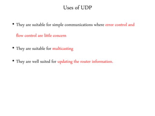
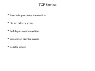
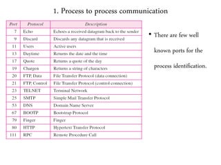
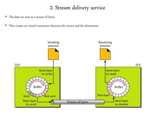
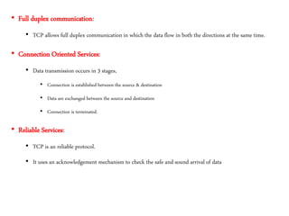
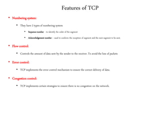
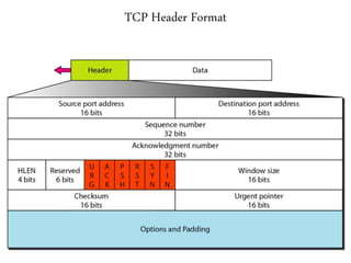
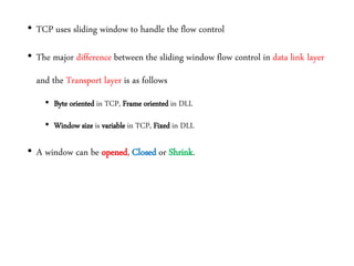
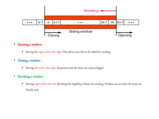
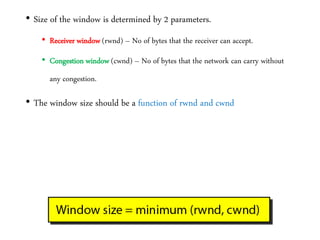
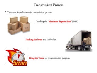
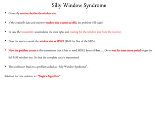
RMK College of Engineering and Technology
CS 6551
Computer Networks
Department
of
Electronics and Communication Engineering
Unit 4
Transport Layer
Prepared by
Jai Ganesh S
Asst.Professor - ECE
Syllabus
• Overview of transport layer
• UDP – User Datagram Protocol
• Reliable Byte Stream – TCP
• Connection management
• Flow control
• Retransmission
• TCP Congestion Control
• Congestion Avoidance
• Quality of Service
• Application Requirements.
Transport Layer
Overview of Transport Layer
• This layer is responsible for process to process delivery of entire message.
• The system runs several process. Transport
layer is responsible for delivering the
message to the correct process.
• This can be achieved by a special type of
address called as “service point address”
IP address vs Port Address
Concept of PORT Addressing
TCP protocols
• There are 2 main protocols used in this layer.
• Connection Less – UDP
• Connection Oriented - TCP
User Datagram Protocol
• This is an connection less un reliable transport layer protocol.
• They have very low error checking features.
UDP packet header
Checksum Calculation
• The UDP check sum has 3 different
sections.
• Pseudo header
• UDP header
• Data from application Layer
Functions of UDP
• Connection less services
• Flow control and error control
• Encapsulation and de capsulation
• Queuing
Uses of UDP
• They are suitable for simple communications where error control and
flow control are little concern
• They are suitable for multicasting
• They are well suited for updating the router information.
End
of
UDP
Reliable Byte Stream
• In contrast to the unreliable transmission protocol we have a reliable byte
stream .
• Protocol used here is “Transmission Control Protocol” (TCP)
TCP Services
• Process to process communication
• Stream delivery service
• Full duplex communication
• Connection oriented service
• Reliable service
1. Process to process communication
• There are few well
known ports for the
process identification.
2. Stream delivery service
• The data are sent as a stream of bytes.
• This creates an virtual connection between the source and the destination.
• Full duplex communication:
• TCP allows full duplex communication in which the data flow in both the directions at the same time.
• Connection Oriented Services:
• Data transmission occurs in 3 stages,
• Connection is established between the source & destination
• Data are exchanged between the source and destination
• Connection is terminated.
• Reliable Services:
• TCP is an reliable protocol.
• It uses an acknowledgement mechanism to check the safe and sound arrival of data
Features of TCP
• Numbering system:
• They have 2 types of numbering system
• Sequence number - to identify the order of the segment
• Acknowledgement number – used to conform the reception of segment and the next segment to be sent.
• Flow control:
• Controls the amount of data sent by the sender to the receiver. To avoid the loss of packets
• Error control:
• TCP implements the error control mechanism to ensure the correct delivery of data.
• Congestion control:
• TCP implements certain strategies to ensure there is no congestion on the network.
TCP Header Format
Connection Management in TCP
• There are 3 phases in connection management.
Connection Establishment
Data transfer
Connection termination
1. Connection Establishment
• Connection is established by a 3
way handshaking process.
• Consider the scenario shown in the
figure, where client need to
establish a connection with the
server.
2. Data transfer
• After the connection is established , data
can flow in bi direction.
• The client and server can send data and
ACK
• The figure shows the timing diagram for
the data transfer phase.
3. Connection Termination
• Connection termination also happens in
3 way handshaking process.
• The client ends the termination by
sending FIN signal and the same is
acknowledged from the server.
End of
Connection Management
Flow Control in TCP
• TCP uses sliding window to handle the flow control
• The major difference between the sliding window flow control in data link layer
and the Transport layer is as follows
• Byte oriented in TCP, Frame oriented in DLL
• Window size is variable in TCP, Fixed in DLL
• A window can be opened, Closed or Shrink.
• Opening a window:
• Moving the right wall to the right. This allows new bits to be added for sending.
• Closing a window:
• Moving left wall to the right. Represents that the bytes are acknowledged.
• Shrinking a window:
• Moving right wall to the left. Revoking the eligibility of bytes for sending. Problem occurs when the bytes are
already sent.
• Size of the window is determined by 2 parameters.
• Receiver window (rwnd) – No of bytes that the receiver can accept.
• Congestion window (cwnd) – No of bytes that the network can carry without
any congestion.
• The window size should be a function of rwnd and cwnd
Transmission Process
• There are 3 mechanisms in transmission process.
Deciding the “Maximum Segment Size” (MSS)
Flushing the bytes into the buffer.
Firing the Timer for retransmission purpose.
Silly Window Syndrome
• Generally receiver decides the window size.
• If the available data and receiver window size is same as MSS, no problem will occur.
• In case the transmitter accumulates the data bytes and waiting for the window size from the receiver.
• Now the receiver sends the window size as MSS/2 (Half the Size of the MSS).
• Now the problem occurs at the transmitter that it has to send MSS/2 bytes of data….. Or to wait for some more period to get the
full MSS window size. So that the complete data is transmitted.
• This confusion leads to a problem called as “Silly Window Syndrome”.
Solution for this problem is : “Nagle’s Algorithm”
• If sender waits too long --> bad for interactive connections.
• If it does not wait long enough --> silly window syndrome.
• How to solve ?
Nagle’sAlgorithm
• If both available data and Window ≥ MSS, send full segment.
• Else, if there is un ACK ed data in flight, buffer new data until ACK
returns.
• Else, send new data now.
End
of
Flow Control
Retransmission
• Reliable data transmission is achieved by retransmitting the
segments.
• The key factor in implementing the retransmission is deciding the
Time Out Period
• The default method for setting up the Time out period
is double the period of Round Trip Time between any 2
nodes on the network
Problem with RTT
• Unfortunately the RTT between any 2 nodes on the network gets varied
because of several factors
Solution
• To eliminate this problem, TCP uses an “Adaptive
Retransmission Technique”.
• Where the Time out Period is adjusted according to the
situations.
• Several algorithms were proposed on calculating the time out period
• Original Algorithm
• Karn / Parteidge Algorithm
• Jacobson / Karels Algorithm
1. Original Algorithm
• This is an simple algorithm, in which the sample time is computed for every segment sent.
• This sample time is related with the previously computed values and the final time out period
is computed as shown below
Drawbacks of Original Algorithm
• RTT cannot be simply calculated only based on the received ACK.
• We cannot identify the received ACK is for the original Transmission or the
Retransmitted Segment
• Consider the given scenarios.
• Case 1: ACK Sent by the Receiver is lost – segment retransmitted – received
ACK is assumed for the original transmission – Sample RTT is too long.
• Case 2: ACK is delayed by the Received – Segment Retransmitted – received
ACK is assumed for the retransmitted segment – Sample RTT is too short.
2. Karn / Parteidge Algorithm
• This algorithm overcomes the drawback of the original algorithm.
• This algorithm proposes that the RTT is computed only for the segments that
are sent for the first time. (Not for the Retransmitted Segments)
• The Final time out is computed based only on the sample RTT’s of first time
sent segments
3. Jacobson / Karels Algorithm
• This algorithm serves better than the predecessor method.
• This algorithm considers the variance of sample RTT’s in to account.
• Variance -- ?
What’s Mean
What’s Variance
End
of
Retransmission
TCP Congestion Control
Congestion Control
• It is very important factor to control the congestion on the network.
• Congestion occurs when the network is overloaded.
• Thus to control the congestion the flow of packets should be controlled according to the
network capacity.
• There are several techniques available. Out of which few techniques are discussed here.
• Adaptive Increase and Multiplicative Decrease.
• Slow Start
• Fast Retransmit and Fast Recovery
Adaptive Increase and Multiplicative Decrease. (AIDM)
• TCP maintains the congestion window size which
decides the amount of data to be transmitted.
• The size of this window can be increased or
decreased according to the occurrence of
congestion on the network.
Operation of AIDM
• AIDM performs slow increase in the congestion
window size when the congestion is less.
• AIDM performs sudden drop in the congestion
window size when there is a congestion on the
network
2. Slow Start Method
• The draw back with the previous method is that, the system take too long time to reach the
optimum flow level.
• This methods initially sets the window size to 1 and when the ACK is received, then it
doubles the window size.
• This method is well suited in 2 conditions
• Initial stage of the transmission when the system do not know anything about the capacity of the
network.
• When the line is down for a while and again back on to service.
Fast retransmit and Fast Recovery
• Fast Retransmit:
• The convention system waits for the time out period to
retransmit the lost frame.
• Instead to speed up the process Fast retransmit is used.
• In this method the receivers send the previous copy of ACK
to the sender to intimate the loss of packets.
• When the receiver keeps on receiving the Duplicate ACK
then the frame is Retransmitted.
Packet 1
Packet 2
Packet 3
Packet 4
Packet 5
Packet 6
Retransmit
packet 3
ACK 1
ACK 2
ACK 2
ACK 2
ACK 6
ACK 2
Sender Receiver
• Fast Recovery:
• This methods modifies the operation of slow start method.
• This methods reduces the size of the congestion window to half, Instead of starting form
the beginning.
• This method helps in fast recovery of the system when there is any occurrence of
congestion in the network.
End
of
Congestion Control
Congestion Avoidance
Introduction
• The previously discussed control mechanisms
measures the amount of congestion occurred in the
network and take steps to control.
• But it is always better to avoid congestion than
controlling.
Congestion avoidance Mechanisms
• There are several congestion avoidance mechanisms proposed. Few of
them are discussed here.
• Destination experiencing Congestion Bit (DEC Bit)
• Random Early Detection (RED).
• Source Based Congestion Avoidance.
DEC Bit
• This system introduces an congestion bit to the packets transmitted by the sender.
• This bit can either set or reset according to the congestion level.
• This bit is set when the queue length if more than 50%.
• When the receiver detects the congestion bit is set then the window size is reduced by 0.875
times the original value.
• When the queue length is less than 50% then the congestion window size is incremented by 1
byte.
Random Early Detection
• This bit avoids congestion by dropping the
packets.
• This method measures the queue length and
fixes minimum threshold and maximum
threshold values.
• When the queue length is below the minimum threshold value then no packets
are dropped.
• When the queue length lies between the minimum and maximum threshold
values then the packets are dropped according to the predefined configuration.
• When the queue length is above the maximum threshold level then all the packets
are dropped.
End
of
Congestion Avoidance
Quality of service (QoS)
QoS - Introduction
• Qos deals with the regular flow of data throughout the network.
• There are several mechanisms incorporated to improve the QoS.
• Scheduling
• Traffic shaping
• Admission control
• Resource reservation.
1. Scheduling
• Scheduling is nothing but prioritizing the various flow of packets.
• There are 3 methods.
• First In First Out Queuing (FIFO)
• Priority Queuing
• Weighted Priority Queuing
FIFO Queuing
Priority Queuing
Weighted Priority Queuing
2. Traffic Shaping
• This method regulates the flow of data from various rates of flow of
packets.
• This can be implemented by 2 techniques.
• Leaky Bucket Mechanism
• Token Bucket Mechanism
Leaky Bucket Mechanism
Leaky Bucket Implementation
Token Bucket Mechanism
• Packets will be sent based on the token system
• Each packet consumes one token.
• The ideal time of the node are effectively utilised in this mechanism
Token Bucket Mechanism
3. Admission Control
• Packets will be accepted or rejected based on the pre defined configuration.
• If the packet passes the test then the packet is accepted. Else rejected.
4. Resource Reservation
• Network resources like bandwidth, queue memory can be reserved before hand for priority
applications .
End
of
QoS
Application Requirements
• It is first important to classify the types of application for choosing the
requirements.
• Real Time Applications
• Non – Real Time Applicaations
Real Time Applications
• The best examples of real time applications are Audio transmission.
• In this applications the minimum delay are most important requirement
than any other parameters.
Non Real time applications
• Such kind of applications do not require minimum delay as the important requirement.
• The parameters like security, correct delivery can be important requirements based on the applications
• Email, FTP and HTTP are few examples of Non Real time Applications.
Approaches for Deciding the QoS
• There are 2 main approaches in providing the QoS.
• Fine Grained Approach
• Provides QoS for individual Applications
• Coarse Grained Approach
• Provides QoS for large class of data or Aggregate Traffic.
End
of
Application Requirements
&
Unit - 4

Computer networks unit iv

  • 1.
    RMK College ofEngineering and Technology CS 6551 Computer Networks Department of Electronics and Communication Engineering
  • 2.
    Unit 4 Transport Layer Preparedby Jai Ganesh S Asst.Professor - ECE
  • 3.
    Syllabus • Overview oftransport layer • UDP – User Datagram Protocol • Reliable Byte Stream – TCP • Connection management • Flow control • Retransmission • TCP Congestion Control • Congestion Avoidance • Quality of Service • Application Requirements.
  • 4.
  • 5.
    Overview of TransportLayer • This layer is responsible for process to process delivery of entire message. • The system runs several process. Transport layer is responsible for delivering the message to the correct process. • This can be achieved by a special type of address called as “service point address”
  • 6.
    IP address vsPort Address
  • 7.
    Concept of PORTAddressing
  • 8.
    TCP protocols • Thereare 2 main protocols used in this layer. • Connection Less – UDP • Connection Oriented - TCP
  • 9.
    User Datagram Protocol •This is an connection less un reliable transport layer protocol. • They have very low error checking features.
  • 10.
  • 11.
    Checksum Calculation • TheUDP check sum has 3 different sections. • Pseudo header • UDP header • Data from application Layer
  • 12.
    Functions of UDP •Connection less services • Flow control and error control • Encapsulation and de capsulation • Queuing
  • 13.
    Uses of UDP •They are suitable for simple communications where error control and flow control are little concern • They are suitable for multicasting • They are well suited for updating the router information.
  • 14.
  • 15.
    Reliable Byte Stream •In contrast to the unreliable transmission protocol we have a reliable byte stream . • Protocol used here is “Transmission Control Protocol” (TCP)
  • 16.
    TCP Services • Processto process communication • Stream delivery service • Full duplex communication • Connection oriented service • Reliable service
  • 17.
    1. Process toprocess communication • There are few well known ports for the process identification.
  • 18.
    2. Stream deliveryservice • The data are sent as a stream of bytes. • This creates an virtual connection between the source and the destination.
  • 19.
    • Full duplexcommunication: • TCP allows full duplex communication in which the data flow in both the directions at the same time. • Connection Oriented Services: • Data transmission occurs in 3 stages, • Connection is established between the source & destination • Data are exchanged between the source and destination • Connection is terminated. • Reliable Services: • TCP is an reliable protocol. • It uses an acknowledgement mechanism to check the safe and sound arrival of data
  • 20.
    Features of TCP •Numbering system: • They have 2 types of numbering system • Sequence number - to identify the order of the segment • Acknowledgement number – used to conform the reception of segment and the next segment to be sent. • Flow control: • Controls the amount of data sent by the sender to the receiver. To avoid the loss of packets • Error control: • TCP implements the error control mechanism to ensure the correct delivery of data. • Congestion control: • TCP implements certain strategies to ensure there is no congestion on the network.
  • 21.
  • 22.
    Connection Management inTCP • There are 3 phases in connection management. Connection Establishment Data transfer Connection termination
  • 23.
    1. Connection Establishment •Connection is established by a 3 way handshaking process. • Consider the scenario shown in the figure, where client need to establish a connection with the server.
  • 24.
    2. Data transfer •After the connection is established , data can flow in bi direction. • The client and server can send data and ACK • The figure shows the timing diagram for the data transfer phase.
  • 25.
    3. Connection Termination •Connection termination also happens in 3 way handshaking process. • The client ends the termination by sending FIN signal and the same is acknowledged from the server.
  • 26.
  • 27.
  • 28.
    • TCP usessliding window to handle the flow control • The major difference between the sliding window flow control in data link layer and the Transport layer is as follows • Byte oriented in TCP, Frame oriented in DLL • Window size is variable in TCP, Fixed in DLL • A window can be opened, Closed or Shrink.
  • 29.
    • Opening awindow: • Moving the right wall to the right. This allows new bits to be added for sending. • Closing a window: • Moving left wall to the right. Represents that the bytes are acknowledged. • Shrinking a window: • Moving right wall to the left. Revoking the eligibility of bytes for sending. Problem occurs when the bytes are already sent.
  • 30.
    • Size ofthe window is determined by 2 parameters. • Receiver window (rwnd) – No of bytes that the receiver can accept. • Congestion window (cwnd) – No of bytes that the network can carry without any congestion. • The window size should be a function of rwnd and cwnd
  • 31.
    Transmission Process • Thereare 3 mechanisms in transmission process. Deciding the “Maximum Segment Size” (MSS) Flushing the bytes into the buffer. Firing the Timer for retransmission purpose.
  • 32.
    Silly Window Syndrome •Generally receiver decides the window size. • If the available data and receiver window size is same as MSS, no problem will occur. • In case the transmitter accumulates the data bytes and waiting for the window size from the receiver. • Now the receiver sends the window size as MSS/2 (Half the Size of the MSS). • Now the problem occurs at the transmitter that it has to send MSS/2 bytes of data….. Or to wait for some more period to get the full MSS window size. So that the complete data is transmitted. • This confusion leads to a problem called as “Silly Window Syndrome”. Solution for this problem is : “Nagle’s Algorithm”
  • 33.
    • If senderwaits too long --> bad for interactive connections. • If it does not wait long enough --> silly window syndrome. • How to solve ?
  • 34.
    Nagle’sAlgorithm • If bothavailable data and Window ≥ MSS, send full segment. • Else, if there is un ACK ed data in flight, buffer new data until ACK returns. • Else, send new data now.
  • 35.
  • 36.
  • 37.
    • Reliable datatransmission is achieved by retransmitting the segments. • The key factor in implementing the retransmission is deciding the Time Out Period • The default method for setting up the Time out period is double the period of Round Trip Time between any 2 nodes on the network
  • 38.
    Problem with RTT •Unfortunately the RTT between any 2 nodes on the network gets varied because of several factors
  • 39.
    Solution • To eliminatethis problem, TCP uses an “Adaptive Retransmission Technique”. • Where the Time out Period is adjusted according to the situations. • Several algorithms were proposed on calculating the time out period • Original Algorithm • Karn / Parteidge Algorithm • Jacobson / Karels Algorithm
  • 40.
    1. Original Algorithm •This is an simple algorithm, in which the sample time is computed for every segment sent. • This sample time is related with the previously computed values and the final time out period is computed as shown below
  • 41.
    Drawbacks of OriginalAlgorithm • RTT cannot be simply calculated only based on the received ACK. • We cannot identify the received ACK is for the original Transmission or the Retransmitted Segment • Consider the given scenarios. • Case 1: ACK Sent by the Receiver is lost – segment retransmitted – received ACK is assumed for the original transmission – Sample RTT is too long. • Case 2: ACK is delayed by the Received – Segment Retransmitted – received ACK is assumed for the retransmitted segment – Sample RTT is too short.
  • 42.
    2. Karn /Parteidge Algorithm • This algorithm overcomes the drawback of the original algorithm. • This algorithm proposes that the RTT is computed only for the segments that are sent for the first time. (Not for the Retransmitted Segments) • The Final time out is computed based only on the sample RTT’s of first time sent segments
  • 43.
    3. Jacobson /Karels Algorithm • This algorithm serves better than the predecessor method. • This algorithm considers the variance of sample RTT’s in to account. • Variance -- ?
  • 44.
  • 45.
  • 47.
  • 48.
  • 49.
    Congestion Control • Itis very important factor to control the congestion on the network. • Congestion occurs when the network is overloaded. • Thus to control the congestion the flow of packets should be controlled according to the network capacity. • There are several techniques available. Out of which few techniques are discussed here. • Adaptive Increase and Multiplicative Decrease. • Slow Start • Fast Retransmit and Fast Recovery
  • 50.
    Adaptive Increase andMultiplicative Decrease. (AIDM) • TCP maintains the congestion window size which decides the amount of data to be transmitted. • The size of this window can be increased or decreased according to the occurrence of congestion on the network.
  • 51.
    Operation of AIDM •AIDM performs slow increase in the congestion window size when the congestion is less. • AIDM performs sudden drop in the congestion window size when there is a congestion on the network
  • 52.
    2. Slow StartMethod • The draw back with the previous method is that, the system take too long time to reach the optimum flow level. • This methods initially sets the window size to 1 and when the ACK is received, then it doubles the window size. • This method is well suited in 2 conditions • Initial stage of the transmission when the system do not know anything about the capacity of the network. • When the line is down for a while and again back on to service.
  • 53.
    Fast retransmit andFast Recovery • Fast Retransmit: • The convention system waits for the time out period to retransmit the lost frame. • Instead to speed up the process Fast retransmit is used. • In this method the receivers send the previous copy of ACK to the sender to intimate the loss of packets. • When the receiver keeps on receiving the Duplicate ACK then the frame is Retransmitted. Packet 1 Packet 2 Packet 3 Packet 4 Packet 5 Packet 6 Retransmit packet 3 ACK 1 ACK 2 ACK 2 ACK 2 ACK 6 ACK 2 Sender Receiver
  • 54.
    • Fast Recovery: •This methods modifies the operation of slow start method. • This methods reduces the size of the congestion window to half, Instead of starting form the beginning. • This method helps in fast recovery of the system when there is any occurrence of congestion in the network.
  • 55.
  • 56.
  • 57.
    Introduction • The previouslydiscussed control mechanisms measures the amount of congestion occurred in the network and take steps to control. • But it is always better to avoid congestion than controlling.
  • 58.
    Congestion avoidance Mechanisms •There are several congestion avoidance mechanisms proposed. Few of them are discussed here. • Destination experiencing Congestion Bit (DEC Bit) • Random Early Detection (RED). • Source Based Congestion Avoidance.
  • 59.
    DEC Bit • Thissystem introduces an congestion bit to the packets transmitted by the sender. • This bit can either set or reset according to the congestion level. • This bit is set when the queue length if more than 50%. • When the receiver detects the congestion bit is set then the window size is reduced by 0.875 times the original value. • When the queue length is less than 50% then the congestion window size is incremented by 1 byte.
  • 60.
    Random Early Detection •This bit avoids congestion by dropping the packets. • This method measures the queue length and fixes minimum threshold and maximum threshold values.
  • 61.
    • When thequeue length is below the minimum threshold value then no packets are dropped. • When the queue length lies between the minimum and maximum threshold values then the packets are dropped according to the predefined configuration. • When the queue length is above the maximum threshold level then all the packets are dropped.
  • 63.
  • 64.
  • 65.
    QoS - Introduction •Qos deals with the regular flow of data throughout the network. • There are several mechanisms incorporated to improve the QoS. • Scheduling • Traffic shaping • Admission control • Resource reservation.
  • 66.
    1. Scheduling • Schedulingis nothing but prioritizing the various flow of packets. • There are 3 methods. • First In First Out Queuing (FIFO) • Priority Queuing • Weighted Priority Queuing
  • 67.
  • 68.
  • 69.
  • 70.
    2. Traffic Shaping •This method regulates the flow of data from various rates of flow of packets. • This can be implemented by 2 techniques. • Leaky Bucket Mechanism • Token Bucket Mechanism
  • 71.
  • 72.
  • 73.
    Token Bucket Mechanism •Packets will be sent based on the token system • Each packet consumes one token. • The ideal time of the node are effectively utilised in this mechanism
  • 74.
  • 75.
    3. Admission Control •Packets will be accepted or rejected based on the pre defined configuration. • If the packet passes the test then the packet is accepted. Else rejected.
  • 76.
    4. Resource Reservation •Network resources like bandwidth, queue memory can be reserved before hand for priority applications .
  • 77.
  • 78.
  • 79.
    Application Requirements • Itis first important to classify the types of application for choosing the requirements. • Real Time Applications • Non – Real Time Applicaations
  • 80.
    Real Time Applications •The best examples of real time applications are Audio transmission. • In this applications the minimum delay are most important requirement than any other parameters.
  • 81.
    Non Real timeapplications • Such kind of applications do not require minimum delay as the important requirement. • The parameters like security, correct delivery can be important requirements based on the applications • Email, FTP and HTTP are few examples of Non Real time Applications.
  • 82.
    Approaches for Decidingthe QoS • There are 2 main approaches in providing the QoS. • Fine Grained Approach • Provides QoS for individual Applications • Coarse Grained Approach • Provides QoS for large class of data or Aggregate Traffic.
  • 83.