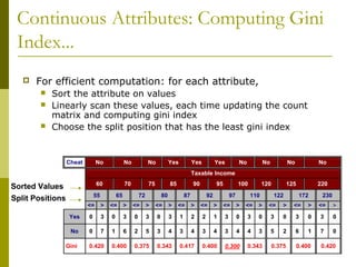
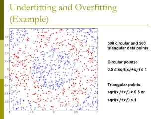
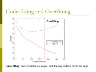
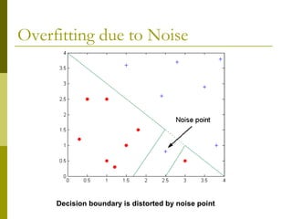
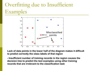
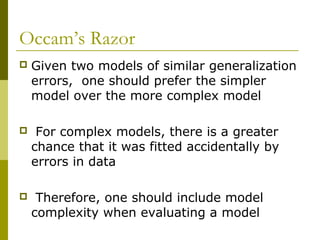
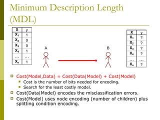
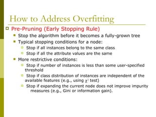
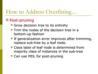
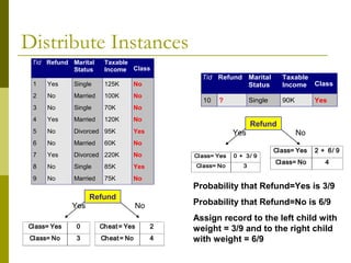
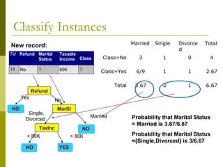
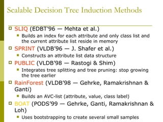
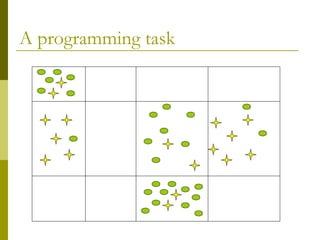
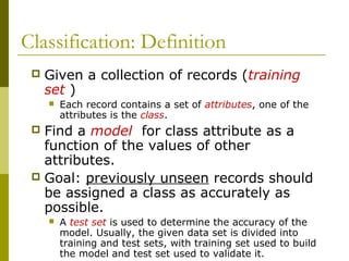
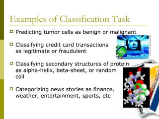
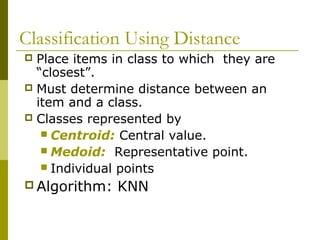
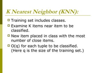
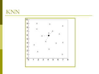
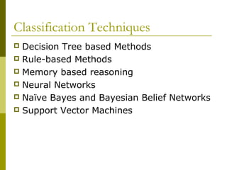
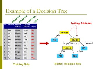
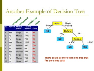
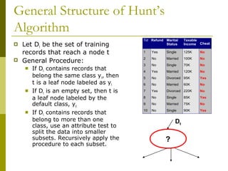
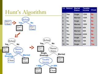
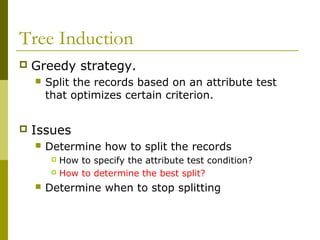
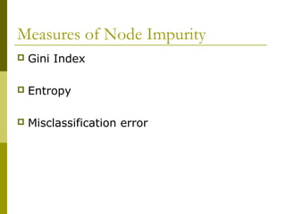
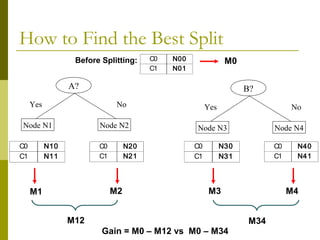
The document discusses the basic concepts of classification and decision trees, detailing the process of classifying records based on their attributes to assign a class label accurately. It covers various classification techniques such as k-nearest neighbors, decision trees, and algorithms like Hunt's, CART, and ID3, providing examples and illustrating the structure and induction of decision trees. Additionally, it explains methods for evaluating splits using criteria like Gini index, entropy, and classification error.

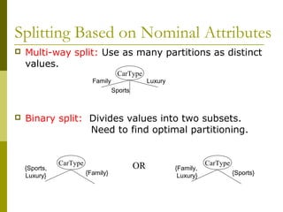
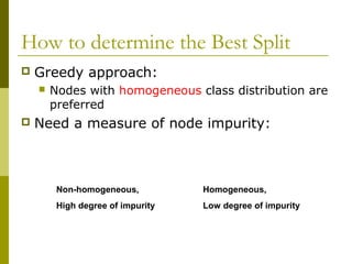
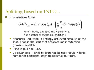
![Measure of Impurity: GINI
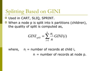
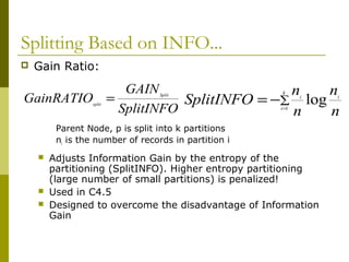
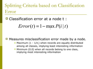
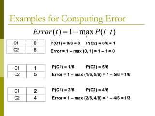
Gini Index for a given node t :
(NOTE: p( j | t) is the relative frequency of class j at node t).
Maximum (1 - 1/nc) when records are equally distributed
among all classes, implying least interesting information
Minimum (0.0) when all records belong to one class,
implying most interesting information
∑−=
j
tjptGINI 2
)]|([1)(
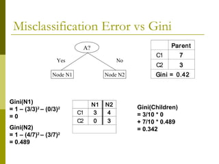
C1 0
C2 6
Gini= 0.000
C1 2
C2 4
Gini= 0.444
C1 3
C2 3
Gini= 0.500
C1 1
C2 5
Gini= 0.278](https://image.slidesharecdn.com/160301117-171130014410/85/Classification-Basic-Concepts-and-Decision-Trees-35-320.jpg)
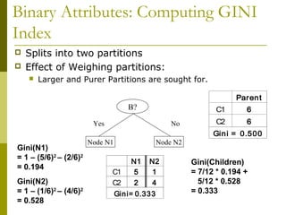
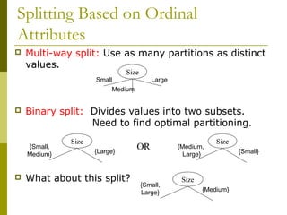
![Examples for computing GINI
C1 0
C2 6
C1 2
C2 4
C1 1
C2 5
P(C1) = 0/6 = 0 P(C2) = 6/6 = 1
Gini = 1 – P(C1)2
– P(C2)2
= 1 – 0 – 1 = 0
∑−=
j
tjptGINI 2
)]|([1)(
P(C1) = 1/6 P(C2) = 5/6
Gini = 1 – (1/6)2
– (5/6)2
= 0.278
P(C1) = 2/6 P(C2) = 4/6
Gini = 1 – (2/6)2
– (4/6)2
= 0.444](https://image.slidesharecdn.com/160301117-171130014410/85/Classification-Basic-Concepts-and-Decision-Trees-36-320.jpg)