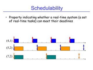
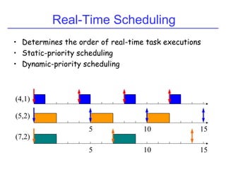
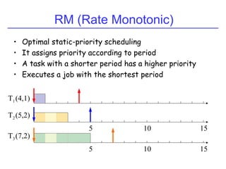
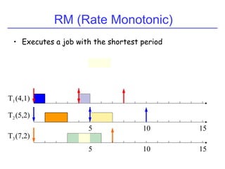
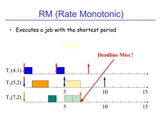
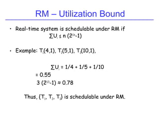
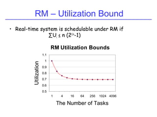
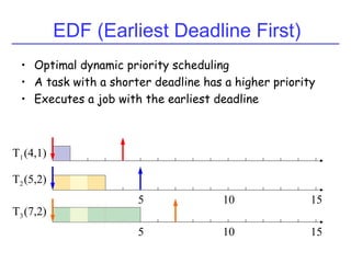
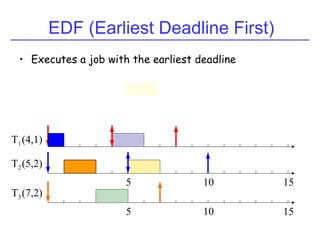
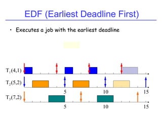
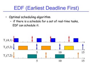
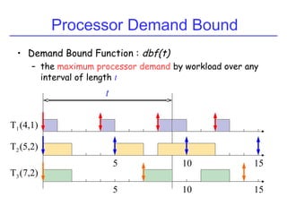
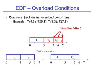
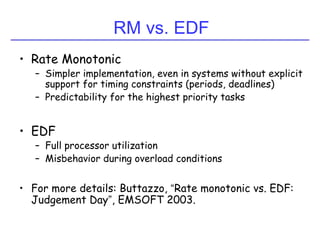
Real-Time Scheduling
CIS700
Insup Lee
By
SATHISHKUMAR G
(sathishsak111@gmail.com)
Outline
• Real-time systems
• Real-time scheduling algorithms
– Fixed-priority algorithm (RM)
– Dynamic-priority algorithm (EDF)
Real-Time Systems
• Definition
– Systems whose correctness depends on their temporal
aspects as well as their functional aspects
• Performance measure
– Timeliness on timing constraints (deadlines)
– Speed/average case performance are less significant.
• Key property
– Predictability on timing constraints
Real-Time System Example
• Digital control systems
– periodically performs the following job:
senses the system status and
actuates the system according to its current status
Control-Law
Computation
Sensor
Actuator
Real-Time System Example
Multimedia
• Multimedia applications
– periodically performs the following job:
reads, decompresses, and displays video and audio
streams
Fundamental Real-Time Issue
• To specify the timing constraints of real-time
systems
• To achieve predictability on satisfying their timing
constraints, possibly, with the existence of other
real-time systems
Scheduling Framework Example
CPU
OS Scheduler
Digital Controller Multimedia
Real-Time Workload
• Job (unit of work)
– a computation, a file read, a message transmission, etc
• Attributes
– Resources required to make progress
– Timing parameters
Released
Absolute
deadline
Relative deadline
Execution time
Real-Time Task
• Task : a sequence of similar jobs
– Periodic task (p,e)
• Its jobs repeat regularly
• Period p = inter-release time (0 < p)
• Execution time e = maximum execution time (0 < e < p)
• Utilization U = e/p
5 10 150
Deadlines: Hard vs. Soft
• Hard deadline
– Disastrous or very serious consequences may occur if
the deadline is missed
– Validation is essential : can all the deadlines be met,
even under worst-case scenario?
– Deterministic guarantees
• Soft deadline
– Ideally, the deadline should be met for maximum
performance. The performance degrades in case of
deadline misses.
– Best effort approaches / statistical guarantees
Schedulability
• Property indicating whether a real-time system (a set
of real-time tasks) can meet their deadlines
(4,1)
(5,2)
(7,2)
Real-Time Scheduling
• Determines the order of real-time task executions
• Static-priority scheduling
• Dynamic-priority scheduling
(4,1)
(5,2)
(7,2)
5
5
10
10 15
15
RM (Rate Monotonic)
• Optimal static-priority scheduling
• It assigns priority according to period
• A task with a shorter period has a higher priority
• Executes a job with the shortest period
(4,1)
(5,2)
(7,2)
5
5
10
10 15
15
T1
T2
T3
RM (Rate Monotonic)
• Executes a job with the shortest period
(4,1)
(5,2)
(7,2)
5
5
10
10 15
15
T1
T2
T3
RM (Rate Monotonic)
• Executes a job with the shortest period
(4,1)
(5,2)
(7,2)
Deadline Miss !
5
5
10
10 15
15
T1
T2
T3
Response Time
• Response time
– Duration from released time to finish time
(4,1)
(5,2)
(10,2)
5
5
10
10 15
15
T1
T2
T3
Response Time
• Response time
– Duration from released time to finish time
(4,1)
(5,2)
(10,2)
Response Time
5
5
10
10 15
15
T1
T2
T3
Response Time
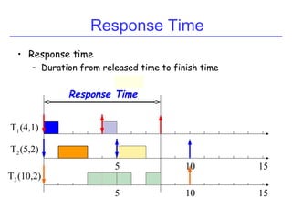
• Response Time (ri) [Audsley et al., 1993]
• HP(Ti) : a set of higher-priority tasks than Ti
(4,1)
(5,2)
(10,2)
k
THPT k
i
ii e
p
r
er
ik
⋅





+= ∑∈ )(
5
5
10
10
T1
T2
T3
RM - Schedulability Analysis
• Real-time system is schedulable under RM
if and only if ri ≤ pi for all task Ti(pi,ei)
Joseph & Pandya,
“Finding response times in a real-time system”,
The Computer Journal, 1986.
RM – Utilization Bound
• Real-time system is schedulable under RM if
∑Ui ≤ n (21/n
-1)
Liu & Layland,
“Scheduling algorithms for multi-programming in a
hard-real-time environment”, Journal of ACM, 1973.
RM – Utilization Bound
• Real-time system is schedulable under RM if
∑Ui ≤ n (21/n
-1)
• Example: T1(4,1), T2(5,1), T3(10,1),
∑Ui = 1/4 + 1/5 + 1/10
= 0.55
3 (21/3
-1) ≈ 0.78
Thus, {T1, T2, T3} is schedulable under RM.
RM Utilization Bounds
0.5
0.6
0.7
0.8
0.9
1
1.1
1 4 16 64 256 1024 4096
The Number of Tasks
Utilization
RM – Utilization Bound
• Real-time system is schedulable under RM if
∑Ui ≤ n (21/n
-1)
EDF (Earliest Deadline First)
• Optimal dynamic priority scheduling
• A task with a shorter deadline has a higher priority
• Executes a job with the earliest deadline
(4,1)
(5,2)
(7,2)
5
5
10
10 15
15
T1
T2
T3
EDF (Earliest Deadline First)
• Executes a job with the earliest deadline
(4,1)
(5,2)
(7,2)
5
5
10
10 15
15
T1
T2
T3
EDF (Earliest Deadline First)
• Executes a job with the earliest deadline
(4,1)
(5,2)
(7,2)
5
5
10
10 15
15
T1
T2
T3
EDF (Earliest Deadline First)
• Executes a job with the earliest deadline
(4,1)
(5,2)
(7,2)
5
5
10
10 15
15
T1
T2
T3
EDF (Earliest Deadline First)
• Optimal scheduling algorithm
– if there is a schedule for a set of real-time tasks,
EDF can schedule it.
(4,1)
(5,2)
(7,2)
5
5
10
10 15
15
T1
T2
T3
Processor Demand Bound
• Demand Bound Function : dbf(t)
– the maximum processor demand by workload over any
interval of length t
(4,1)
(5,2)
(7,2)
t
5
5
10
10 15
15
T1
T2
T3
EDF - Schedulability Analysis
• Real-time system is schedulable under EDF
if and only if dbf(t) ≤ t for all interval t
Baruah et al.
“Algorithms and complexity concerning the preemptive
scheduling of periodic, real-time tasks on one
processor”, Journal of Real-Time Systems, 1990.
• Demand Bound Function : dbf(t)
– the maximum processor demand by workload over any
interval of length t
EDF – Utilization Bound
• Real-time system is schedulable under EDF if and only
if
∑Ui ≤ 1
Liu & Layland,
“Scheduling algorithms for multi-programming in a
hard-real-time environment”, Journal of ACM, 1973.
• Domino effect during overload conditions
– Example: T1(4,3), T2(5,3), T3(6,3), T4(7,3)
EDF – Overload Conditions
T1
50 7
T2 T3 T4
3 6
Deadline Miss !
T1
50 7
T3
3 6
Better schedules :
T1
50 7
T4
3 6
RM vs. EDF
• Rate Monotonic
– Simpler implementation, even in systems without explicit
support for timing constraints (periods, deadlines)
– Predictability for the highest priority tasks
• EDF
– Full processor utilization
– Misbehavior during overload conditions
• For more details: Buttazzo, “Rate monotonic vs. EDF:
Judgement Day”, EMSOFT 2003.
THANK YOU

Real-Time Scheduling

  • 1.
  • 2.
    Outline • Real-time systems •Real-time scheduling algorithms – Fixed-priority algorithm (RM) – Dynamic-priority algorithm (EDF)
  • 3.
    Real-Time Systems • Definition –Systems whose correctness depends on their temporal aspects as well as their functional aspects • Performance measure – Timeliness on timing constraints (deadlines) – Speed/average case performance are less significant. • Key property – Predictability on timing constraints
  • 4.
    Real-Time System Example •Digital control systems – periodically performs the following job: senses the system status and actuates the system according to its current status Control-Law Computation Sensor Actuator
  • 5.
    Real-Time System Example Multimedia •Multimedia applications – periodically performs the following job: reads, decompresses, and displays video and audio streams
  • 6.
    Fundamental Real-Time Issue •To specify the timing constraints of real-time systems • To achieve predictability on satisfying their timing constraints, possibly, with the existence of other real-time systems
  • 7.
    Scheduling Framework Example CPU OSScheduler Digital Controller Multimedia
  • 8.
    Real-Time Workload • Job(unit of work) – a computation, a file read, a message transmission, etc • Attributes – Resources required to make progress – Timing parameters Released Absolute deadline Relative deadline Execution time
  • 9.
    Real-Time Task • Task: a sequence of similar jobs – Periodic task (p,e) • Its jobs repeat regularly • Period p = inter-release time (0 < p) • Execution time e = maximum execution time (0 < e < p) • Utilization U = e/p 5 10 150
  • 10.
    Deadlines: Hard vs.Soft • Hard deadline – Disastrous or very serious consequences may occur if the deadline is missed – Validation is essential : can all the deadlines be met, even under worst-case scenario? – Deterministic guarantees • Soft deadline – Ideally, the deadline should be met for maximum performance. The performance degrades in case of deadline misses. – Best effort approaches / statistical guarantees
  • 11.
    Schedulability • Property indicatingwhether a real-time system (a set of real-time tasks) can meet their deadlines (4,1) (5,2) (7,2)
  • 12.
    Real-Time Scheduling • Determinesthe order of real-time task executions • Static-priority scheduling • Dynamic-priority scheduling (4,1) (5,2) (7,2) 5 5 10 10 15 15
  • 13.
    RM (Rate Monotonic) •Optimal static-priority scheduling • It assigns priority according to period • A task with a shorter period has a higher priority • Executes a job with the shortest period (4,1) (5,2) (7,2) 5 5 10 10 15 15 T1 T2 T3
  • 14.
    RM (Rate Monotonic) •Executes a job with the shortest period (4,1) (5,2) (7,2) 5 5 10 10 15 15 T1 T2 T3
  • 15.
    RM (Rate Monotonic) •Executes a job with the shortest period (4,1) (5,2) (7,2) Deadline Miss ! 5 5 10 10 15 15 T1 T2 T3
  • 16.
    Response Time • Responsetime – Duration from released time to finish time (4,1) (5,2) (10,2) 5 5 10 10 15 15 T1 T2 T3
  • 17.
    Response Time • Responsetime – Duration from released time to finish time (4,1) (5,2) (10,2) Response Time 5 5 10 10 15 15 T1 T2 T3
  • 18.
    Response Time • ResponseTime (ri) [Audsley et al., 1993] • HP(Ti) : a set of higher-priority tasks than Ti (4,1) (5,2) (10,2) k THPT k i ii e p r er ik ⋅      += ∑∈ )( 5 5 10 10 T1 T2 T3
  • 19.
    RM - SchedulabilityAnalysis • Real-time system is schedulable under RM if and only if ri ≤ pi for all task Ti(pi,ei) Joseph & Pandya, “Finding response times in a real-time system”, The Computer Journal, 1986.
  • 20.
    RM – UtilizationBound • Real-time system is schedulable under RM if ∑Ui ≤ n (21/n -1) Liu & Layland, “Scheduling algorithms for multi-programming in a hard-real-time environment”, Journal of ACM, 1973.
  • 21.
    RM – UtilizationBound • Real-time system is schedulable under RM if ∑Ui ≤ n (21/n -1) • Example: T1(4,1), T2(5,1), T3(10,1), ∑Ui = 1/4 + 1/5 + 1/10 = 0.55 3 (21/3 -1) ≈ 0.78 Thus, {T1, T2, T3} is schedulable under RM.
  • 22.
    RM Utilization Bounds 0.5 0.6 0.7 0.8 0.9 1 1.1 14 16 64 256 1024 4096 The Number of Tasks Utilization RM – Utilization Bound • Real-time system is schedulable under RM if ∑Ui ≤ n (21/n -1)
  • 23.
    EDF (Earliest DeadlineFirst) • Optimal dynamic priority scheduling • A task with a shorter deadline has a higher priority • Executes a job with the earliest deadline (4,1) (5,2) (7,2) 5 5 10 10 15 15 T1 T2 T3
  • 24.
    EDF (Earliest DeadlineFirst) • Executes a job with the earliest deadline (4,1) (5,2) (7,2) 5 5 10 10 15 15 T1 T2 T3
  • 25.
    EDF (Earliest DeadlineFirst) • Executes a job with the earliest deadline (4,1) (5,2) (7,2) 5 5 10 10 15 15 T1 T2 T3
  • 26.
    EDF (Earliest DeadlineFirst) • Executes a job with the earliest deadline (4,1) (5,2) (7,2) 5 5 10 10 15 15 T1 T2 T3
  • 27.
    EDF (Earliest DeadlineFirst) • Optimal scheduling algorithm – if there is a schedule for a set of real-time tasks, EDF can schedule it. (4,1) (5,2) (7,2) 5 5 10 10 15 15 T1 T2 T3
  • 28.
    Processor Demand Bound •Demand Bound Function : dbf(t) – the maximum processor demand by workload over any interval of length t (4,1) (5,2) (7,2) t 5 5 10 10 15 15 T1 T2 T3
  • 29.
    EDF - SchedulabilityAnalysis • Real-time system is schedulable under EDF if and only if dbf(t) ≤ t for all interval t Baruah et al. “Algorithms and complexity concerning the preemptive scheduling of periodic, real-time tasks on one processor”, Journal of Real-Time Systems, 1990. • Demand Bound Function : dbf(t) – the maximum processor demand by workload over any interval of length t
  • 30.
    EDF – UtilizationBound • Real-time system is schedulable under EDF if and only if ∑Ui ≤ 1 Liu & Layland, “Scheduling algorithms for multi-programming in a hard-real-time environment”, Journal of ACM, 1973.
  • 31.
    • Domino effectduring overload conditions – Example: T1(4,3), T2(5,3), T3(6,3), T4(7,3) EDF – Overload Conditions T1 50 7 T2 T3 T4 3 6 Deadline Miss ! T1 50 7 T3 3 6 Better schedules : T1 50 7 T4 3 6
  • 32.
    RM vs. EDF •Rate Monotonic – Simpler implementation, even in systems without explicit support for timing constraints (periods, deadlines) – Predictability for the highest priority tasks • EDF – Full processor utilization – Misbehavior during overload conditions • For more details: Buttazzo, “Rate monotonic vs. EDF: Judgement Day”, EMSOFT 2003.
  • 33.