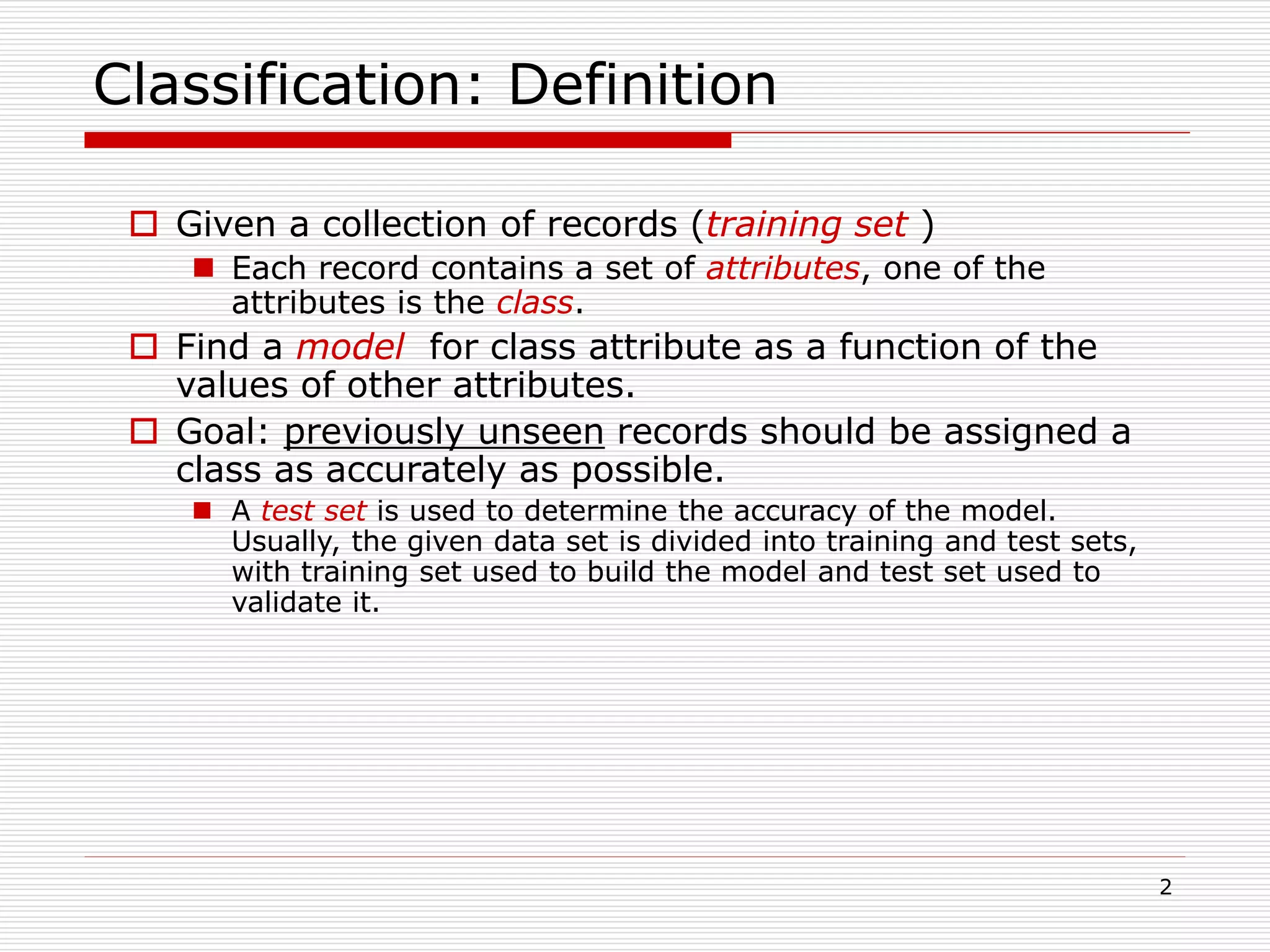
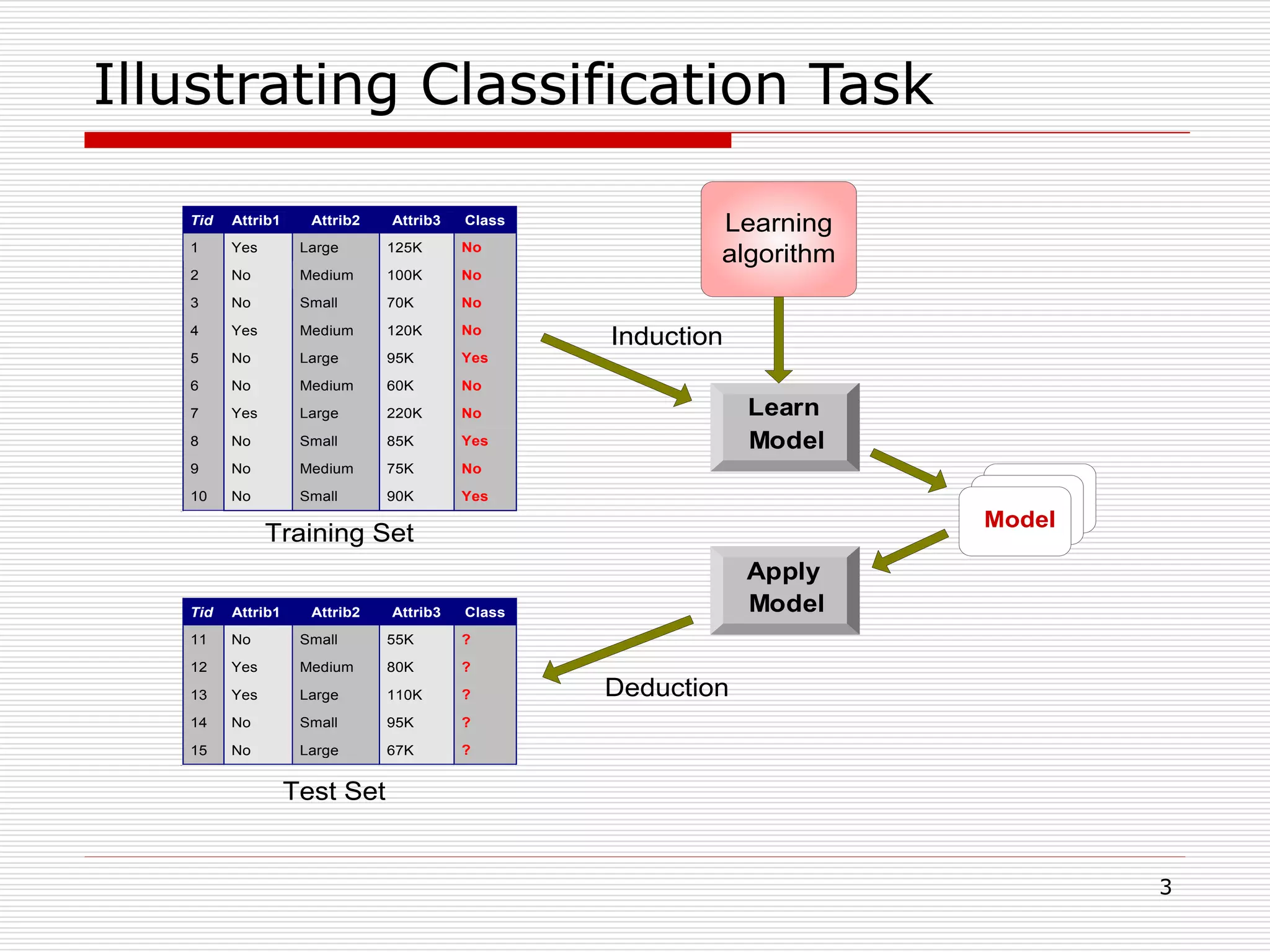
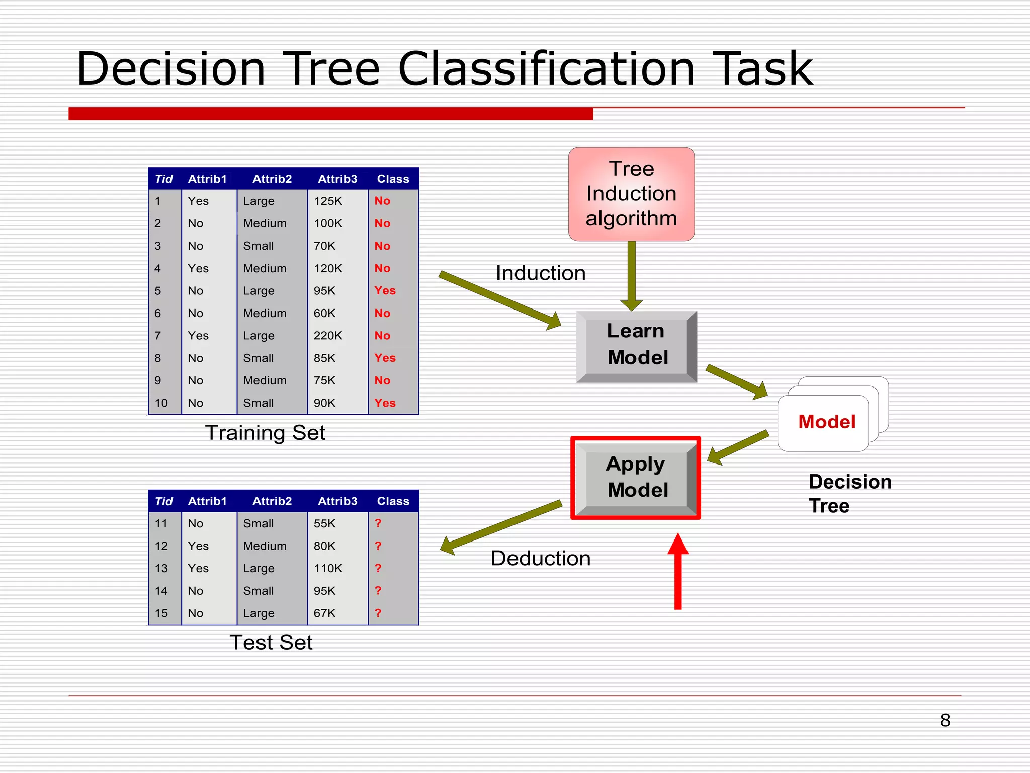
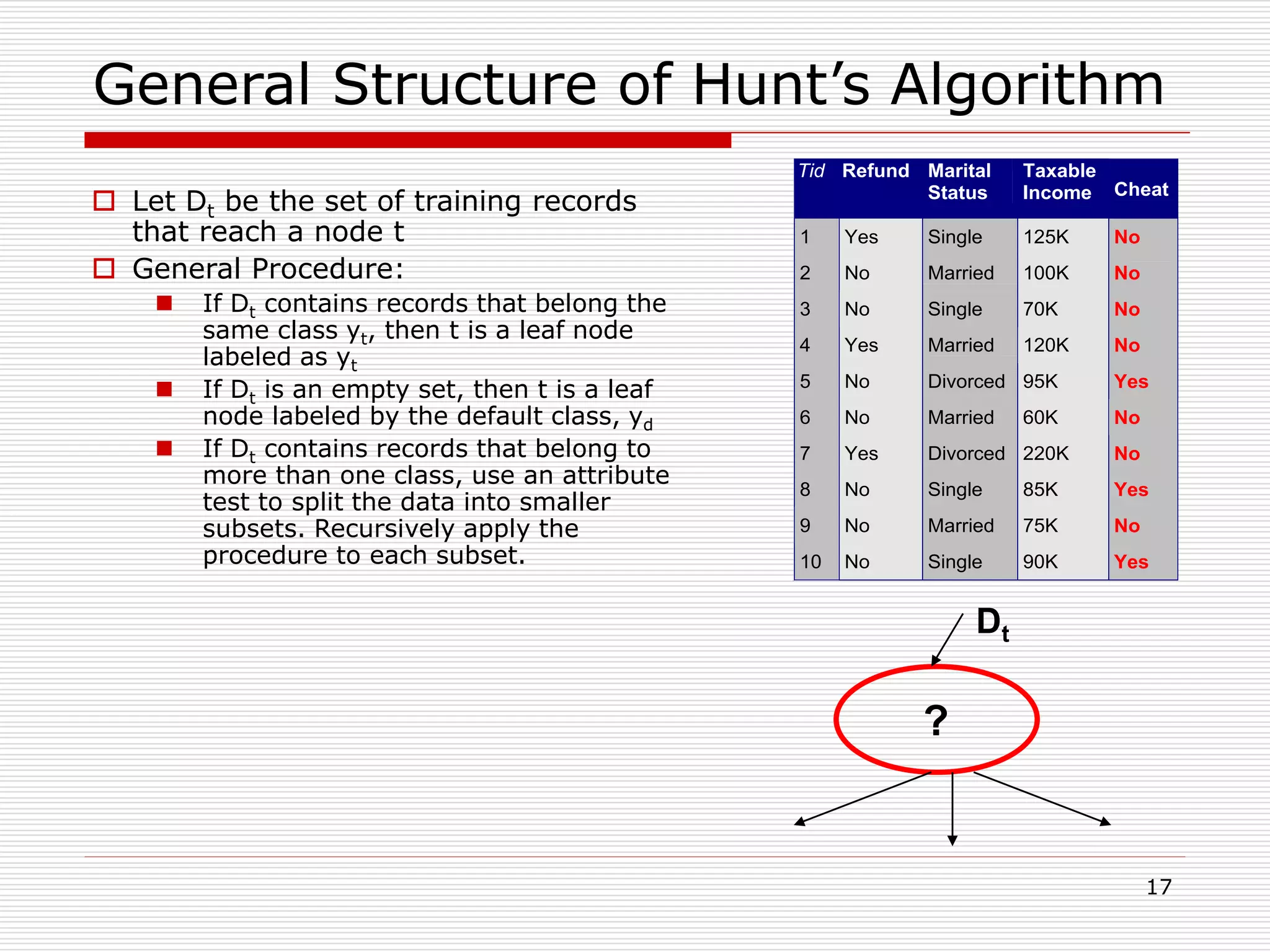
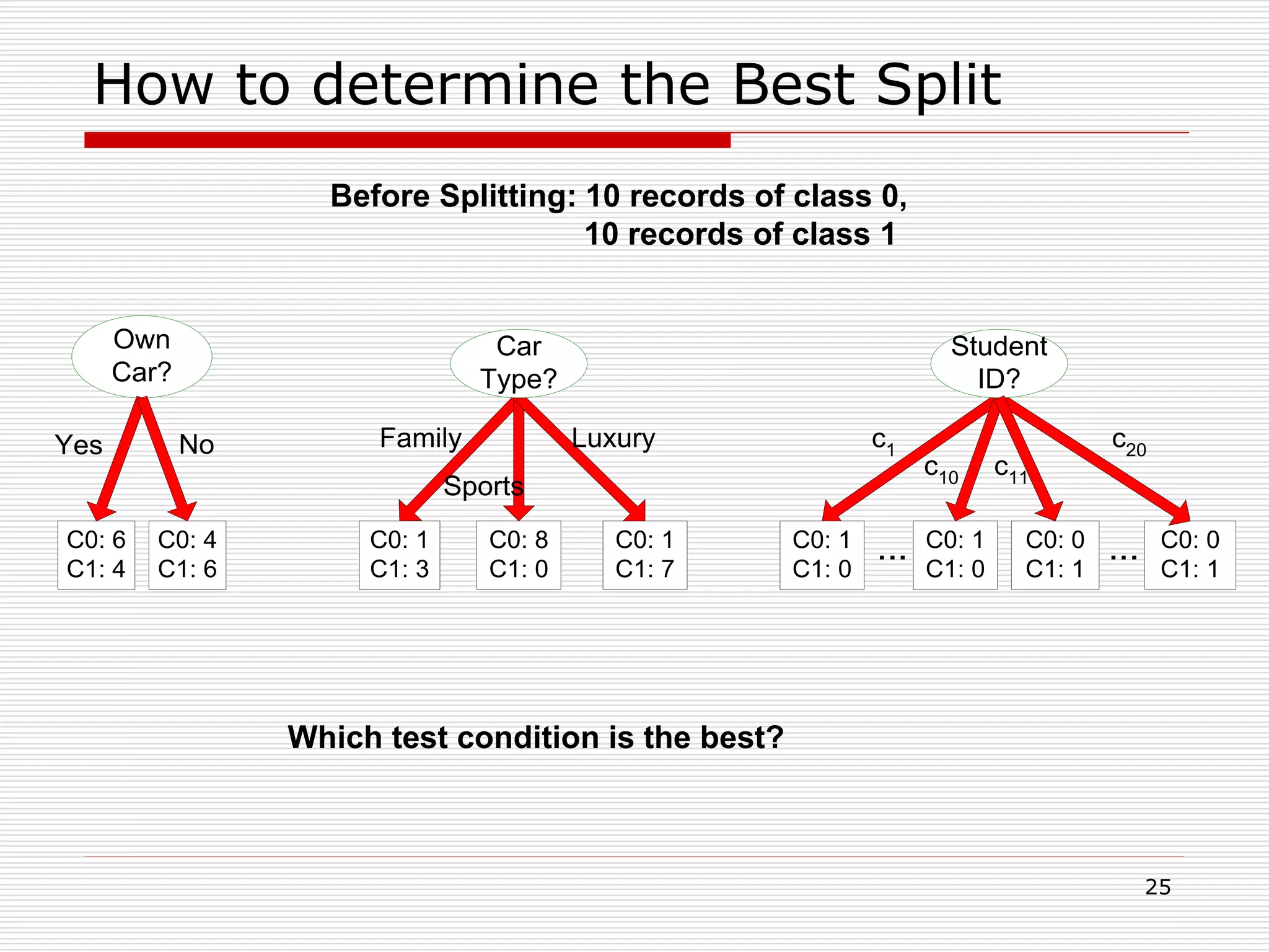
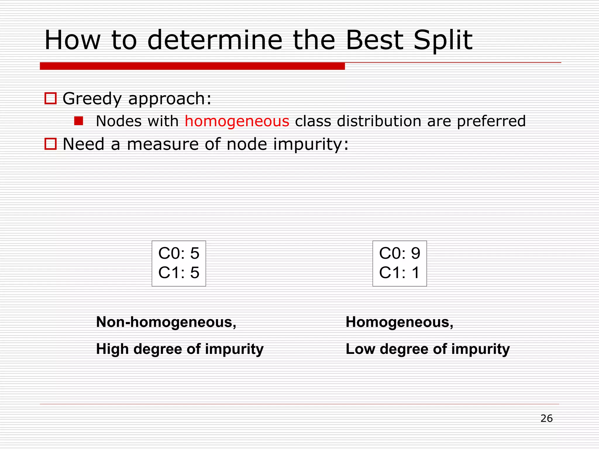
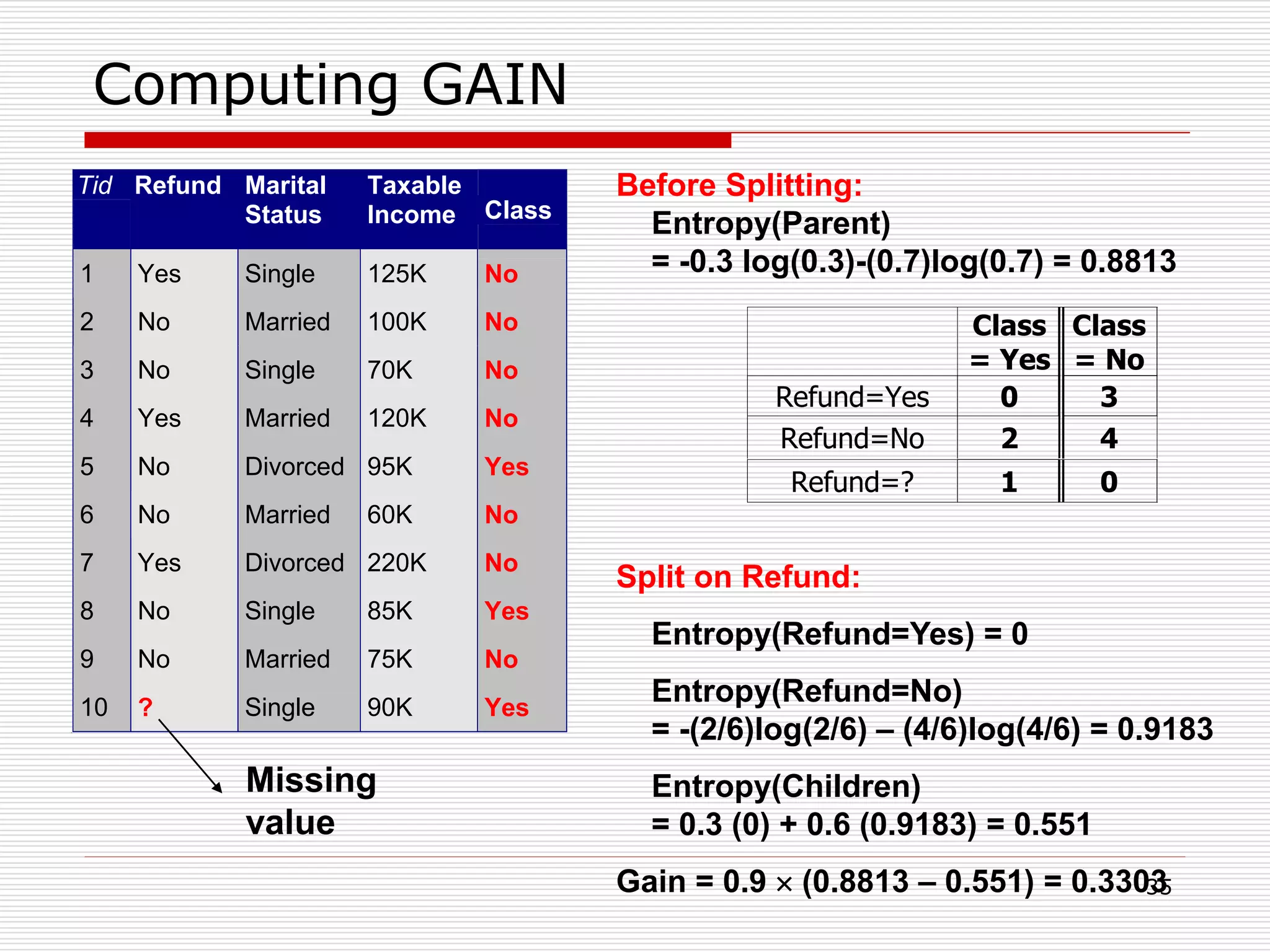
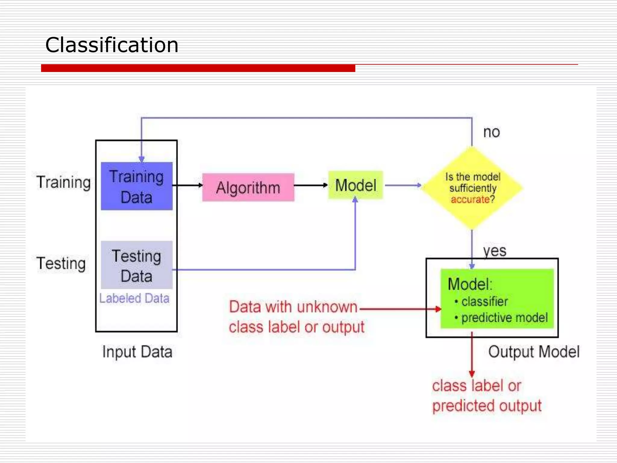
Classification is a supervised machine learning task where a model is trained on labeled data to predict the class labels of new unlabeled data. The given document discusses classification and decision tree induction for classification. It defines classification, provides examples of classification tasks, and describes how decision trees are constructed through a greedy top-down induction approach that aims to split the training data into homogeneous subsets based on measures of impurity like Gini index or information gain. The goal is to build an accurate model that can classify new unlabeled data.

1. Modul 6:
Classification

2. 2
Classification: Definition
 Given a collection of records (training set )
 Each record contains a set of attributes, one of the
attributes is the class.
 Find a model for class attribute as a function of the
values of other attributes.
 Goal: previously unseen records should be assigned a
class as accurately as possible.
 A test set is used to determine the accuracy of the model.
Usually, the given data set is divided into training and test sets,
with training set used to build the model and test set used to
validate it.

3. 3
Illustrating Classification Task
Apply
Model
Induction
Deduction
Learn
Model
Model
Tid Attrib1 Attrib2 Attrib3 Class
1 Yes Large 125K No
2 No Medium 100K No
3 No Small 70K No
4 Yes Medium 120K No
5 No Large 95K Yes
6 No Medium 60K No
7 Yes Large 220K No
8 No Small 85K Yes
9 No Medium 75K No
10 No Small 90K Yes
10
Tid Attrib1 Attrib2 Attrib3 Class
11 No Small 55K ?
12 Yes Medium 80K ?
13 Yes Large 110K ?
14 No Small 95K ?
15 No Large 67K ?
10
Test Set
Learning
algorithm
Training Set

4. 4
Examples of Classification Task
 Predicting tumor cells as benign or malignant
 Classifying credit card transactions
as legitimate or fraudulent
 Classifying secondary structures of protein
as alpha-helix, beta-sheet, or random
coil
 Categorizing news stories as finance,
weather, entertainment, sports, etc

5. 5
Classification Techniques
 Decision Tree based Methods
 Rule-based Methods
 Memory based reasoning
 Neural Networks
 Naïve Bayes and Bayesian Belief Networks
 Support Vector Machines

6. 6
Example of a Decision Tree
Tid Refund Marital
Status
Taxable
Income Cheat
1 Yes Single 125K No
2 No Married 100K No
3 No Single 70K No
4 Yes Married 120K No
5 No Divorced 95K Yes
6 No Married 60K No
7 Yes Divorced 220K No
8 No Single 85K Yes
9 No Married 75K No
10 No Single 90K Yes
10
Refund
MarSt
TaxInc
YESNO
NO
NO
Yes No
MarriedSingle, Divorced
< 80K > 80K
Splitting Attributes
Training Data Model: Decision Tree

7. 7
Another Example of Decision Tree
Tid Refund Marital
Status
Taxable
Income Cheat
1 Yes Single 125K No
2 No Married 100K No
3 No Single 70K No
4 Yes Married 120K No
5 No Divorced 95K Yes
6 No Married 60K No
7 Yes Divorced 220K No
8 No Single 85K Yes
9 No Married 75K No
10 No Single 90K Yes
10
MarSt
Refund
TaxInc
YESNO
NO
NO
Yes No
Married
Single,
Divorced
< 80K > 80K
There could be more than one tree that
fits the same data!

8. 8
Decision Tree Classification Task
Apply
Model
Induction
Deduction
Learn
Model
Model
Tid Attrib1 Attrib2 Attrib3 Class
1 Yes Large 125K No
2 No Medium 100K No
3 No Small 70K No
4 Yes Medium 120K No
5 No Large 95K Yes
6 No Medium 60K No
7 Yes Large 220K No
8 No Small 85K Yes
9 No Medium 75K No
10 No Small 90K Yes
10
Tid Attrib1 Attrib2 Attrib3 Class
11 No Small 55K ?
12 Yes Medium 80K ?
13 Yes Large 110K ?
14 No Small 95K ?
15 No Large 67K ?
10
Test Set
Tree
Induction
algorithm
Training Set
Decision
Tree

9. 9
Apply Model to Test Data
Refund
MarSt
TaxInc
YESNO
NO
NO
Yes No
MarriedSingle, Divorced
< 80K > 80K
Refund Marital
Status
Taxable
Income Cheat
No Married 80K ?
10
Test Data
Start from the root of tree.

10. 10
Apply Model to Test Data
Refund
MarSt
TaxInc
YESNO
NO
NO
Yes No
MarriedSingle, Divorced
< 80K > 80K
Refund Marital
Status
Taxable
Income Cheat
No Married 80K ?
10
Test Data

11. 11
Apply Model to Test Data
Refund
MarSt
TaxInc
YESNO
NO
NO
Yes No
MarriedSingle, Divorced
< 80K > 80K
Refund Marital
Status
Taxable
Income Cheat
No Married 80K ?
10
Test Data

12. 12
Apply Model to Test Data
Refund
MarSt
TaxInc
YESNO
NO
NO
Yes No
MarriedSingle, Divorced
< 80K > 80K
Refund Marital
Status
Taxable
Income Cheat
No Married 80K ?
10
Test Data

13. 13
Apply Model to Test Data
Refund
MarSt
TaxInc
YESNO
NO
NO
Yes No
MarriedSingle, Divorced
< 80K > 80K
Refund Marital
Status
Taxable
Income Cheat
No Married 80K ?
10
Test Data

14. 14
Apply Model to Test Data
Refund
MarSt
TaxInc
YESNO
NO
NO
Yes No
MarriedSingle, Divorced
< 80K > 80K
Refund Marital
Status
Taxable
Income Cheat
No Married 80K ?
10
Test Data
Assign Cheat to “No”

15. 15
Decision Tree Classification Task
Apply
Model
Induction
Deduction
Learn
Model
Model
Tid Attrib1 Attrib2 Attrib3 Class
1 Yes Large 125K No
2 No Medium 100K No
3 No Small 70K No
4 Yes Medium 120K No
5 No Large 95K Yes
6 No Medium 60K No
7 Yes Large 220K No
8 No Small 85K Yes
9 No Medium 75K No
10 No Small 90K Yes
10
Tid Attrib1 Attrib2 Attrib3 Class
11 No Small 55K ?
12 Yes Medium 80K ?
13 Yes Large 110K ?
14 No Small 95K ?
15 No Large 67K ?
10
Test Set
Tree
Induction
algorithm
Training Set
Decision
Tree

16. 16
Decision Tree Induction
 Many Algorithms:
 Hunt’s Algorithm (one of the earliest)
 CART
 ID3, C4.5
 SLIQ,SPRINT

17. 17
General Structure of Hunt’s Algorithm
 Let Dt be the set of training records
that reach a node t
 General Procedure:
 If Dt contains records that belong the
same class yt, then t is a leaf node
labeled as yt
 If Dt is an empty set, then t is a leaf
node labeled by the default class, yd
 If Dt contains records that belong to
more than one class, use an attribute
test to split the data into smaller
subsets. Recursively apply the
procedure to each subset.
Tid Refund Marital
Status
Taxable
Income Cheat
1 Yes Single 125K No
2 No Married 100K No
3 No Single 70K No
4 Yes Married 120K No
5 No Divorced 95K Yes
6 No Married 60K No
7 Yes Divorced 220K No
8 No Single 85K Yes
9 No Married 75K No
10 No Single 90K Yes
10
Dt
?

18. 18
Hunt’s Algorithm
Don’t
Cheat
Refund
Don’t
Cheat
Don’t
Cheat
Yes No
Refund
Don’t
Cheat
Yes No
Marital
Status
Don’t
Cheat
Cheat
Single,
Divorced
Married
Taxable
Income
Don’t
Cheat
< 80K >= 80K
Refund
Don’t
Cheat
Yes No
Marital
Status
Don’t
Cheat
Cheat
Single,
Divorced
Married
Tid Refund Marital
Status
Taxable
Income Cheat
1 Yes Single 125K No
2 No Married 100K No
3 No Single 70K No
4 Yes Married 120K No
5 No Divorced 95K Yes
6 No Married 60K No
7 Yes Divorced 220K No
8 No Single 85K Yes
9 No Married 75K No
10 No Single 90K Yes
10

19. 19
Tree Induction
 Greedy strategy.
 Split the records based on an attribute test that optimizes
certain criterion.
 Issues
 Determine how to split the records
 How to specify the attribute test condition?
 How to determine the best split?
 Determine when to stop splitting

20. 20
How to Specify Test Condition?
 Depends on attribute types
 Nominal
 Ordinal
 Continuous
 Depends on number of ways to split
 2-way split
 Multi-way split

21. 21
Splitting Based on Nominal Attributes
 Multi-way split: Use as many partitions as distinct values.
 Binary split: Divides values into two subsets.
Need to find optimal partitioning.
CarType
Family
Sports
Luxury
CarType
{Family,
Luxury} {Sports}
CarType
{Sports,
Luxury} {Family} OR

22. 22
 Multi-way split: Use as many partitions as distinct values.
 Binary split: Divides values into two subsets.
Need to find optimal partitioning.
 What about this split?
Splitting Based on Ordinal Attributes
Size
Small
Medium
Large
Size
{Medium,
Large} {Small}Size
{Small,
Medium} {Large}
OR
Size
{Small,
Large} {Medium}

23. 23
Splitting Based on Continuous Attributes
 Different ways of handling
 Discretization to form an ordinal categorical attribute
 Static – discretize once at the beginning
 Dynamic – ranges can be found by equal interval
bucketing, equal frequency bucketing
(percentiles), or clustering.
 Binary Decision: (A < v) or (A  v)
 consider all possible splits and finds the best cut
 can be more compute intensive

24. 24
Splitting Based on Continuous Attributes
Taxable
Income
> 80K?
Yes No
Taxable
Income?
(i) Binary split (ii) Multi-way split
< 10K
[10K,25K) [25K,50K) [50K,80K)
> 80K

25. 25
How to determine the Best Split
Own
Car?
C0: 6
C1: 4
C0: 4
C1: 6
C0: 1
C1: 3
C0: 8
C1: 0
C0: 1
C1: 7
Car
Type?
C0: 1
C1: 0
C0: 1
C1: 0
C0: 0
C1: 1
Student
ID?
...
Yes No Family
Sports
Luxury c1
c10
c20
C0: 0
C1: 1
...
c11
Before Splitting: 10 records of class 0,
10 records of class 1
Which test condition is the best?

26. 26
How to determine the Best Split
 Greedy approach:
 Nodes with homogeneous class distribution are preferred
 Need a measure of node impurity:
C0: 5
C1: 5
C0: 9
C1: 1
Non-homogeneous,
High degree of impurity
Homogeneous,
Low degree of impurity

27. 27
Measures of Node Impurity
 Gini Index
 Entropy
 Misclassification error

28. 28
Measure of Impurity: GINI
 Gini Index for a given node t :
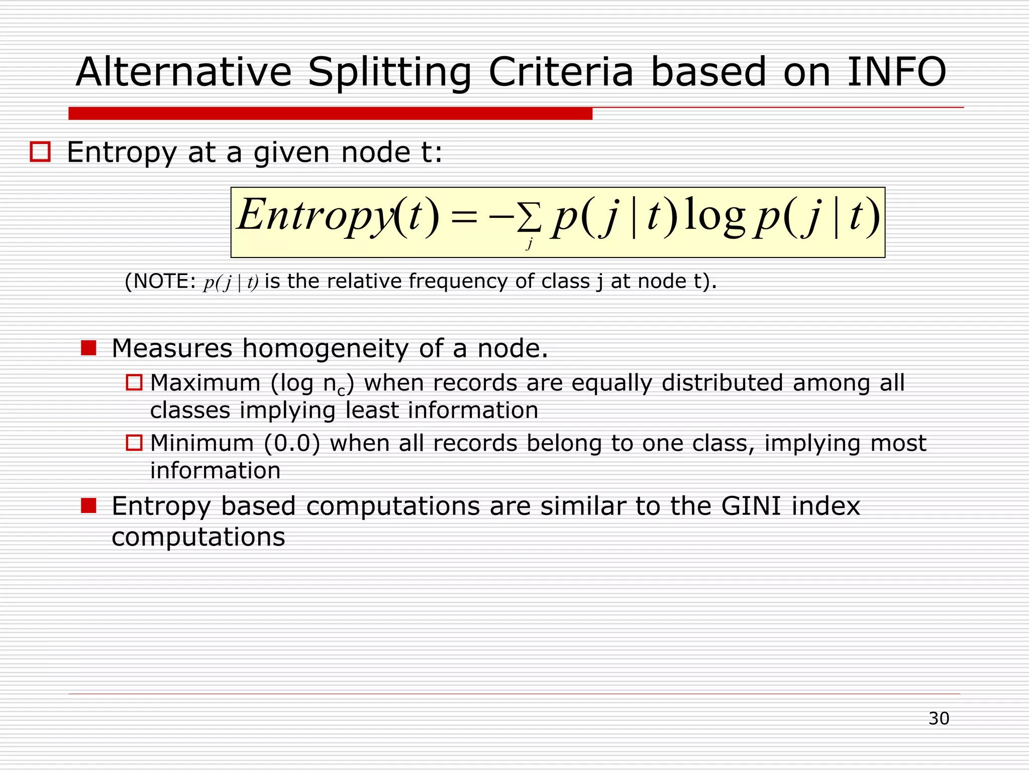
(NOTE: p( j | t) is the relative frequency of class j at node t).
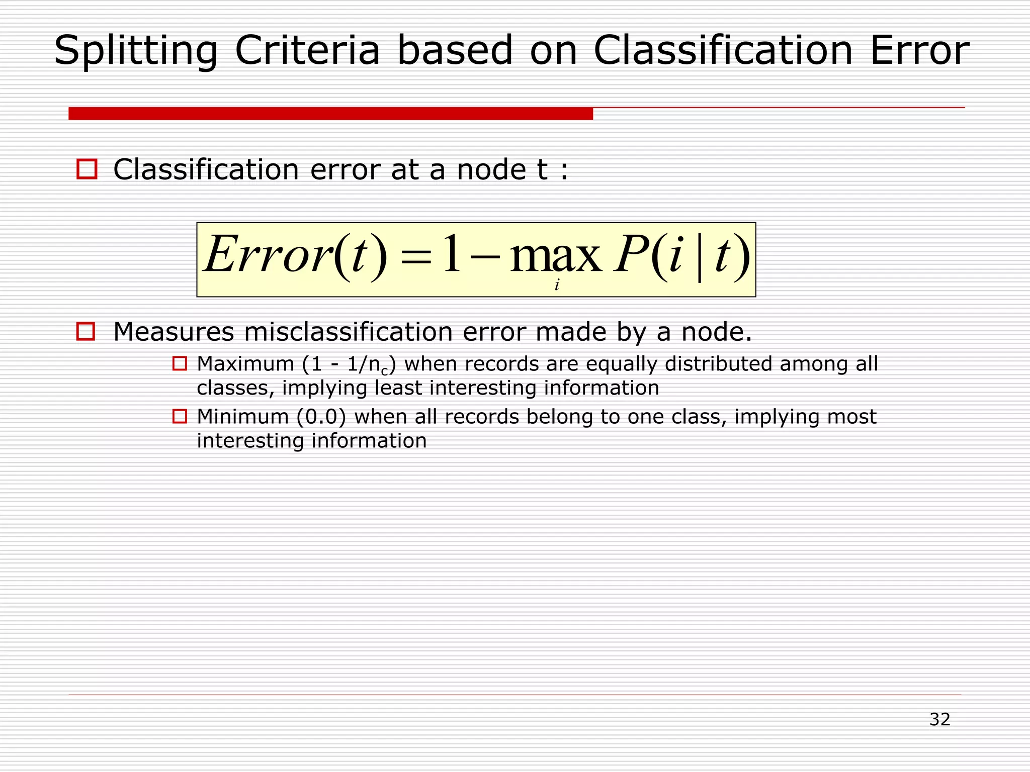
 Maximum (1 - 1/nc) when records are equally distributed among all
classes, implying least interesting information
 Minimum (0.0) when all records belong to one class, implying most
interesting information

j
tjptGINI 2
)]|([1)(
C1 0
C2 6
Gini=0.000
C1 2
C2 4
Gini=0.444
C1 3
C2 3
Gini=0.500
C1 1
C2 5
Gini=0.278

29. 29
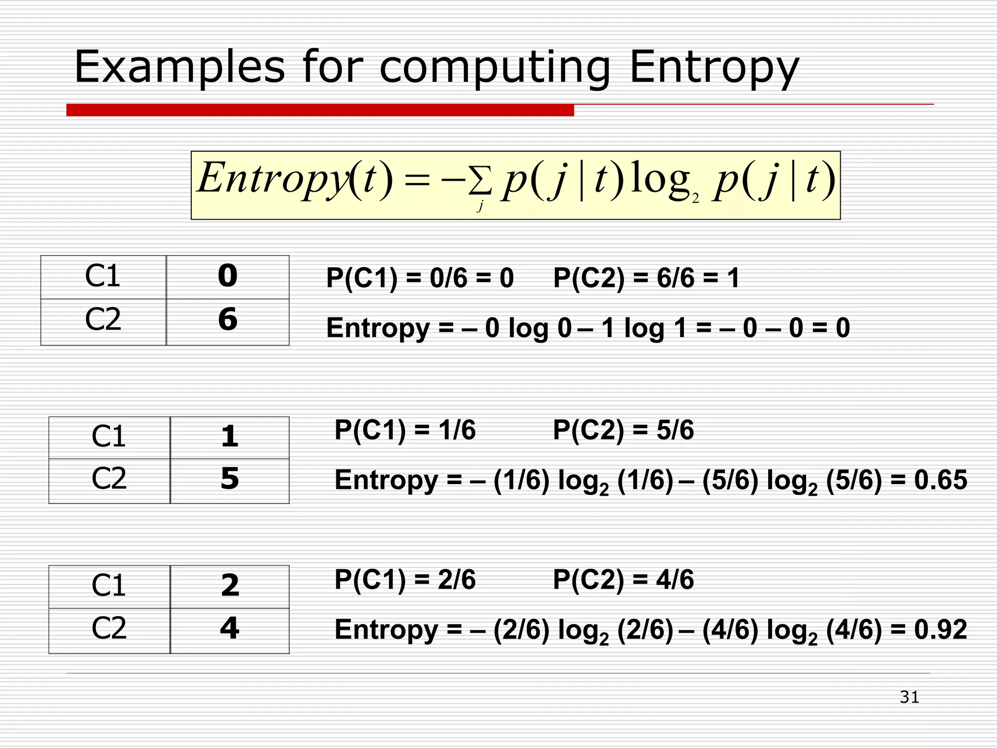
Examples for computing GINI
C1 0
C2 6
C1 2
C2 4
C1 1
C2 5
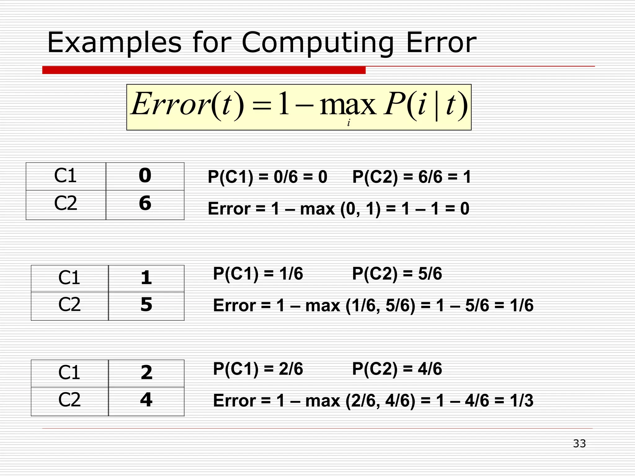
P(C1) = 0/6 = 0 P(C2) = 6/6 = 1
Gini = 1 – P(C1)2 – P(C2)2 = 1 – 0 – 1 = 0

j
tjptGINI 2
)]|([1)(
P(C1) = 1/6 P(C2) = 5/6
Gini = 1 – (1/6)2 – (5/6)2 = 0.278
P(C1) = 2/6 P(C2) = 4/6
Gini = 1 – (2/6)2 – (4/6)2 = 0.444

30. 30
Alternative Splitting Criteria based on INFO
 Entropy at a given node t:
(NOTE: p( j | t) is the relative frequency of class j at node t).
 Measures homogeneity of a node.
 Maximum (log nc) when records are equally distributed among all
classes implying least information
 Minimum (0.0) when all records belong to one class, implying most
information
 Entropy based computations are similar to the GINI index
computations
 j
tjptjptEntropy )|(log)|()(

31. 31
Examples for computing Entropy
C1 0
C2 6
C1 2
C2 4
C1 1
C2 5
P(C1) = 0/6 = 0 P(C2) = 6/6 = 1
Entropy = – 0 log 0 – 1 log 1 = – 0 – 0 = 0
P(C1) = 1/6 P(C2) = 5/6
Entropy = – (1/6) log2 (1/6) – (5/6) log2 (5/6) = 0.65
P(C1) = 2/6 P(C2) = 4/6
Entropy = – (2/6) log2 (2/6) – (4/6) log2 (4/6) = 0.92
 j
tjptjptEntropy )|(log)|()( 2

32. 32
Splitting Criteria based on Classification Error
 Classification error at a node t :
 Measures misclassification error made by a node.
 Maximum (1 - 1/nc) when records are equally distributed among all
classes, implying least interesting information
 Minimum (0.0) when all records belong to one class, implying most
interesting information
)|(max1)( tiPtError i


33. 33
Examples for Computing Error
C1 0
C2 6
C1 2
C2 4
C1 1
C2 5
P(C1) = 0/6 = 0 P(C2) = 6/6 = 1
Error = 1 – max (0, 1) = 1 – 1 = 0
P(C1) = 1/6 P(C2) = 5/6
Error = 1 – max (1/6, 5/6) = 1 – 5/6 = 1/6
P(C1) = 2/6 P(C2) = 4/6
Error = 1 – max (2/6, 4/6) = 1 – 4/6 = 1/3
)|(max1)( tiPtError i


34. 34
Example: Splitting Based on ENTROPY
 Information Gain:
Parent Node, p is split into k partitions;
ni is number of records in partition i
 Measures Reduction in Entropy achieved because of the split.
Choose the split that achieves most reduction (maximizes
GAIN)
 Goal: maximize the GAIN
 Used in ID3 and C4.5
 Disadvantage: Tends to prefer splits that result in large number
of partitions, each being small but pure.






 

k
i
i
split
iEntropy
n
n
pEntropyGAIN 1
)()(

35. 35
Computing GAIN
Tid Refund Marital
Status
Taxable
Income Class
1 Yes Single 125K No
2 No Married 100K No
3 No Single 70K No
4 Yes Married 120K No
5 No Divorced 95K Yes
6 No Married 60K No
7 Yes Divorced 220K No
8 No Single 85K Yes
9 No Married 75K No
10 ? Single 90K Yes
10
Class
= Yes
Class
= No
Refund=Yes 0 3
Refund=No 2 4
Refund=? 1 0
Split on Refund:
Entropy(Refund=Yes) = 0
Entropy(Refund=No)
= -(2/6)log(2/6) – (4/6)log(4/6) = 0.9183
Entropy(Children)
= 0.3 (0) + 0.6 (0.9183) = 0.551
Gain = 0.9  (0.8813 – 0.551) = 0.3303
Missing
value
Before Splitting:
Entropy(Parent)
= -0.3 log(0.3)-(0.7)log(0.7) = 0.8813

36. 36
Splitting Based on ENTROPY
 Gain Ratio:
Parent Node, p is split into k partitions
ni is the number of records in partition i
 Adjusts Information Gain by the entropy of the partitioning
(SplitINFO). Higher entropy partitioning (large number of small
partitions) is penalized!
 Used in C4.5
 Designed to overcome the disadvantage of Information Gain
SplitINFO
GAIN
GainRATIO Split
split
 


k
i
ii
n
n
n
n
SplitINFO 1
log

37. 37
Stopping Criteria for Tree Induction
 Stop expanding a node when all the records belong to the
same class
 Stop expanding a node when all the records have similar
attribute values
 Early termination

38. 38
Decision Tree Based Classification
 Advantages:
 Inexpensive to construct
 Extremely fast at classifying unknown records
 Easy to interpret for small-sized trees
 Accuracy is comparable to other classification techniques for
many simple data sets

39. 39
Example: C4.5
 Simple depth-first construction.
 Uses Information Gain
 Sorts Continuous Attributes at each node.
 Needs entire data to fit in memory.
 Unsuitable for Large Datasets.
 Needs out-of-core sorting.
 You can download the software from:
http://www.cse.unsw.edu.au/~quinlan/c4.5r8.tar.gz

40. Demo: Using C5
(www.rulequest.com)

41. 41
What is See5
 Data mining software for classification
 Technique: decision tree
 Decision tree algorithm: C5.0

42. 42
Sample applications using See5
 Predicting Magnetic Properties of Crystals
 To develop rules that predict whether a substance is magnetic
or not (National Research Council Canada)
 24641 cases, 120 attributes/case
 Profiling High Income Earners from Census Data
 To predict whether the individual's income is above or below
$50,000 (US Census Bureau Database)
 200,000 cases, 40 attributes/cases (7 numeric, 33 nominal
atts)

43. 43
Classification

44. 44
Preparing data for See5

45. 45
Preparing data for See5
 Files used in See5 have names of the form filestem.extension

46. 46
Preparing data for See5
 Content of a hypothyroid.names file

47. 47
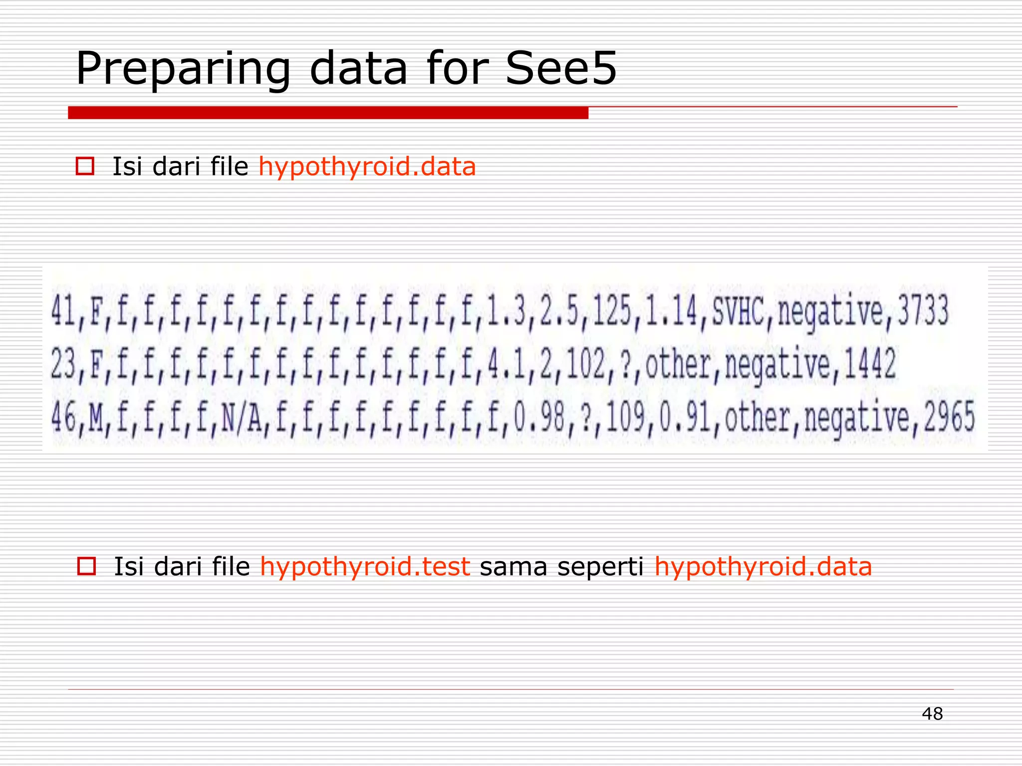
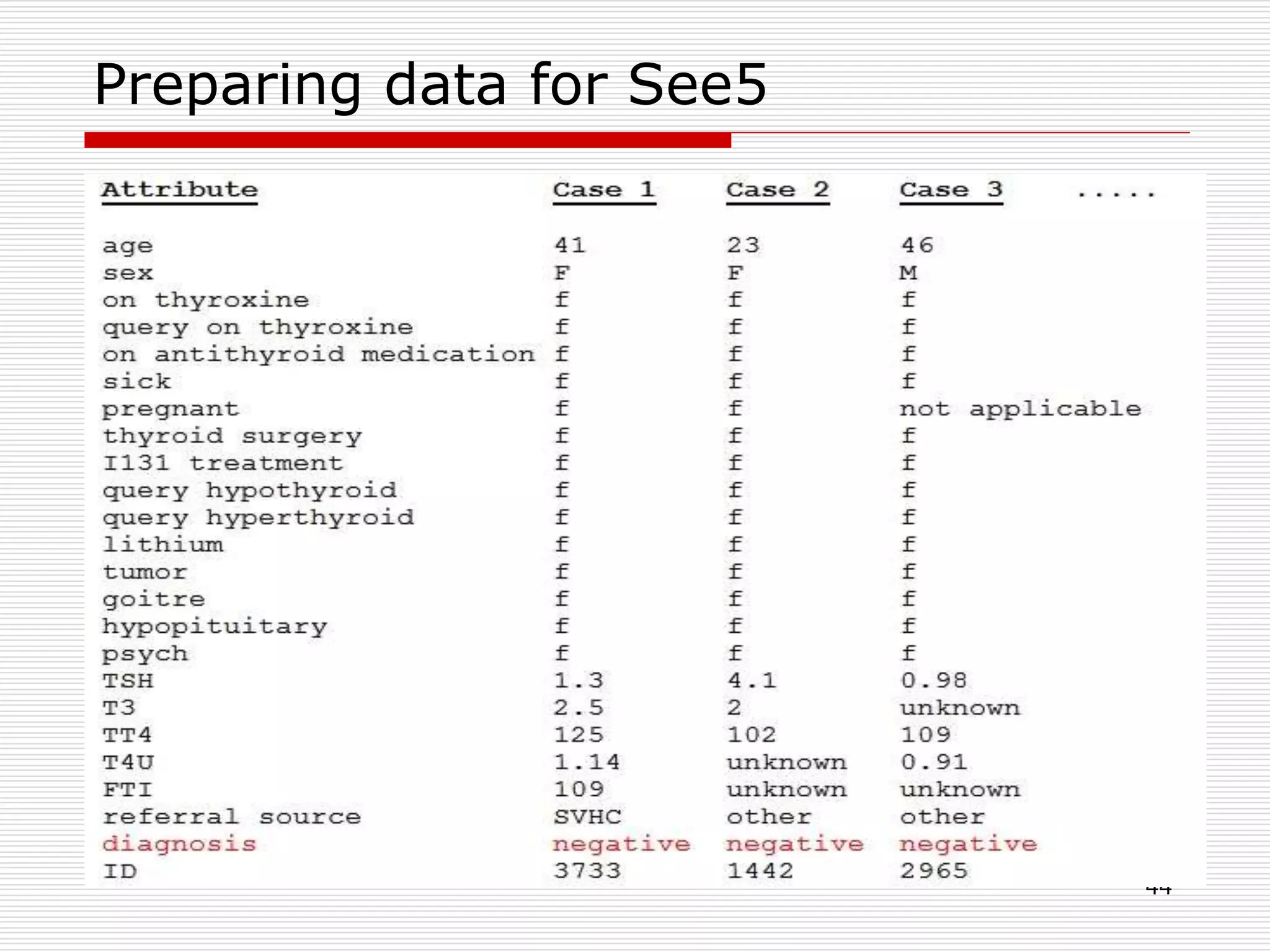
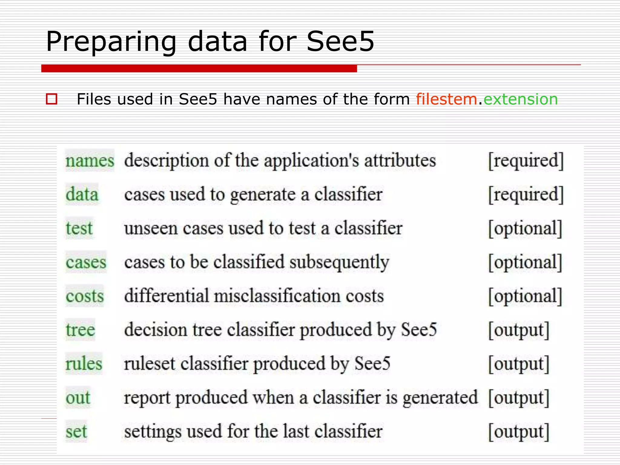
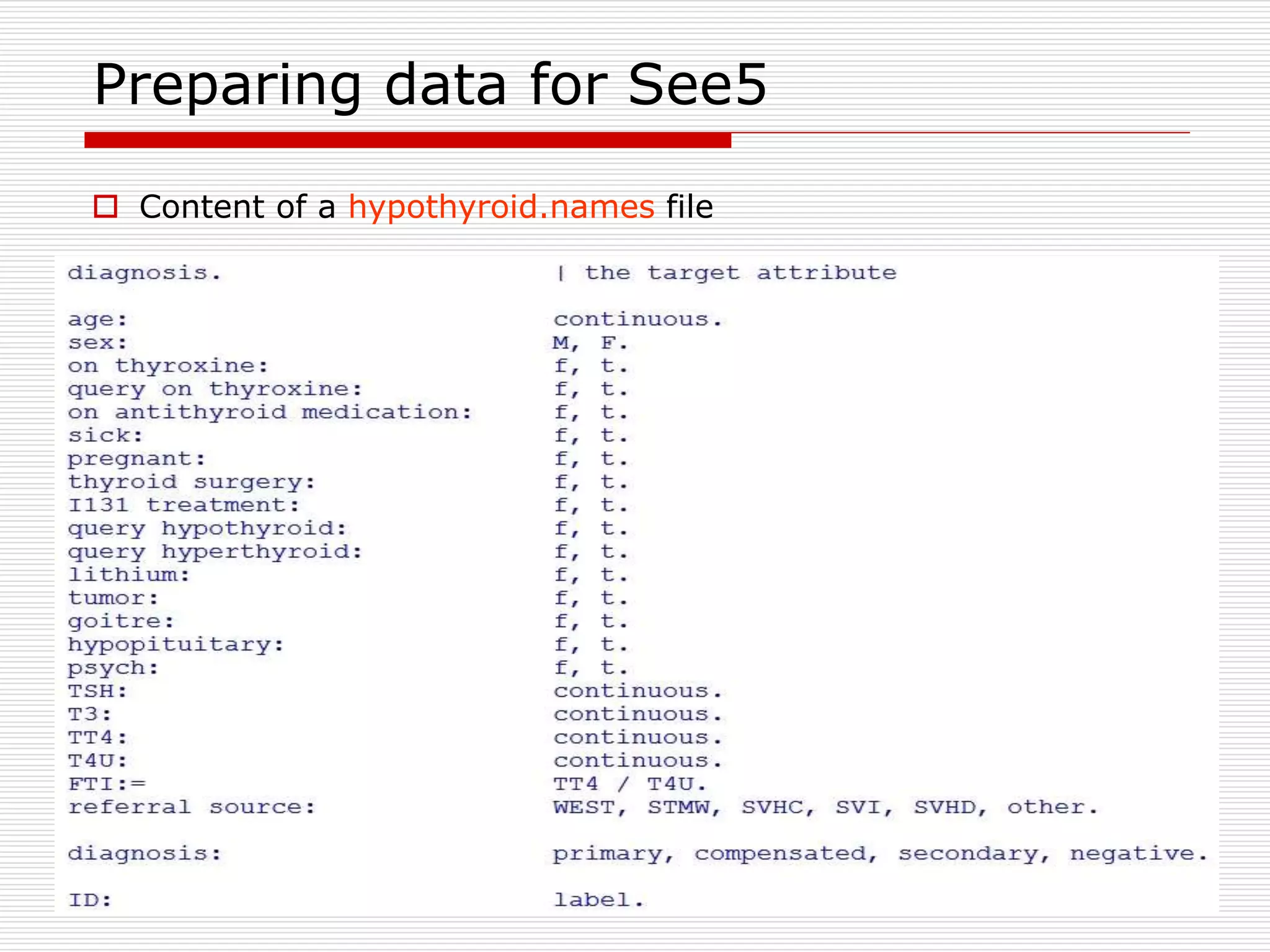
Preparing data for See5
 Types of attributes
 Continuous: numeric values
 Date: dates in the form YYYY/MM/DD or YYYY-MM-DD
 Time: times in the form HH:MM:SS
 Timestamp: times in the form YYYY/MM/DD HH:MM:SS
 Discrete N: discrete, unordered values. N is the maximum
values
 A comma-separated list of names: discrete values
 [ordered] can be used to indicate that the ordering
 Example: grade: [ordered] low, medium, high.
 Label
 Ignore

48. 48
Preparing data for See5
 Isi dari file hypothyroid.data
 Isi dari file hypothyroid.test sama seperti hypothyroid.data

49. 49
See5 GUI

50. 50
Constructing Classifier
 Classifier construction
options:

51. 51
Decision Tree

52. 52
Decision Tree

53. 53
Decision Tree Evaluation
Num. of leaves: 14
Misclassified: 7
Confusion matrix

54. 54
Tree Construction Options
 Discrete value subsets
 Group attribute values into subsets and each subtree is
associated with a subset rather than with a single value.
 Example:
 referral source in {WEST,STMW,SVHC,SVI,SVHD}: primary
(4.9/0.8)

55. 55
Tree Construction Options
 Rulesets
 generate classifiers called rulesets that consist of unordered
collections of (relatively) simple if-then rules.
 Example:

56. 56
 Each rule consists of
 A rule number
 Statistics (n, lift x)
or (n/m, lift x)
 One or more conditions
 A class predicted by
the rule
 A confidence
 Laplace ratio
(n-m+1)/(n+2)

57. 57
Tree Construction Options
 Boosting
 generate several classifiers
(either decision trees or
rulesets) rather than just
one.
 When a new case is to be
classified, each classifier
votes for its predicted class
and the votes are counted
to determine the final
class.
 Example:
 Boost: 10 trials

58. 58
Tree Construction Options
 Winnow
 To choose a subset of the attributes that will be used to
construct the decision tree or ruleset.
 Example:

59. 59
Using Classifier
 Used to predict the classes to which new cases belong.
 Since the values of all attributes may not be needed, the
attribute values requested will depend on the case itself.
 Example: