The document discusses various classification and prediction techniques used in machine learning, including decision trees, naive Bayes classification, and k-nearest neighbors. It provides examples of how these techniques work and compares supervised versus unsupervised learning approaches. The document also covers issues around preparing data and comparing different classification and prediction methods.

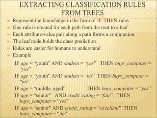
1. CLASSIFICATION
BY
P.LAXMI
UNIT - III

2. WHAT IS CLASSIFICATION? WHAT IS
PREDICTION?

4. EXAMPLES

5. HOW DOES CLASSIFICATION WORK?

7. SUPERVISED VS. UNSUPERVISED LEARNING
 Supervised learning (classification)
 Supervision: The training data (observations, measurements,
etc.) are accompanied by labels indicating the class of the
observations
 New data is classified based on the training set
 Unsupervised learning (clustering)
 The class labels of training data is unknown
 Given a set of measurements, observations, etc. with the aim of
establishing the existence of classes or clusters in the data

8. HOW IS (NUMERIC ) PREDICTION
DIFFERENT FROM CLASSIFICATION?

9. ISSUES REGARDING CLASSIFICATION AND
PREDICTION
1. Preparing the data for classification and prediction

10. 2. Comparing Classification and Prediction Methods

11. CLASSIFICATION BY DECISION TREE
INDUCTION
 Decision tree induction is the learning of decision trees from class-
labeled training tuples.
 A decision tree is a flowchart like tree structure where
 each internal node(non-leaf node) denotes a test on an attribute
 each branch represents an outcome of the test
 each leaf node (terminal node) holds a class label
 The topmost node in a tree is the root node
 Internal nodes are represented by rectangles
 leaf nodes are represented by ovals

12. HOW ARE DECISION TREES USED FOR
CLASSIFICATION
 Given a tuple X, for which class label is unknown, the attribute
values of the tuple are tested against the decision tree.
 A path is traced from root to leaf node, which holds the class
prediction for that tuple.

13. DECISION TREE INDUCTION
 The decision tree induction algorithms are:
 ID3 (Iterative Dichotomiser)
 C4.5 (a successor of ID3)
 CART (Classification and Regression Trees)

15. SPLITTING CRITERION
The splitting criterion indicates the splitting attribute and may also indicate
either a split-point or a splitting subset.

18. STOPPING CRITERIA
 Each leaf node contains examples of one type
 Algorithm ran out of attributes
 No further significant information gain

19. EXAMPLE

20. GAIN RATIO (C4.5)
 The C4.5 algorithm introduces a number of improvements over
the original ID3 algorithm.
 The C4.5 algorithm can handle missing data.
 If the training records contain unknown attribute values, the C4.5
evaluates the gain for an attribute by considering only the records
where the attribute is defined.
 Both categorical and continuous attributes are supported by C4.5
 Values of continuous variable are sorted and partitioned
 For the corresponding records of each partition, the gain is
calculated, and the partition that maximizes the gain is chosen for
the next split.
 The Id3 algorithm may construct a deep and complex tree, which
would cause overfitting.
 The C4.5 algorithm addresses the overfitting problem in ID3 by
using a bottom-up technique called pruning to simplify the tree by
removing the least visited nodes and branches.

21. EXAMPLE
Similarly, find gain ratios for other attributes (age, student, credit_rating)
and the attribute with maximum gain ratio is selected as the splitting
attribute.

22. INDUCTION OF DECISION TREE USING GINI INDEX
(CART)

23. GINI INDEX CALCULATION
 Let D be the training data of Table, where there are nine tuples
belonging to the class buys computer = yes and the remaining five
tuples belong to the class buys computer = no. A (root) node N is
created for the tuples in D.
 Gini index to compute the impurity of D:
 Gini(D) = 1 – (9/14)2 – (5/14)2
 To find the splitting criterion for the tuples in D, we need to
compute the gini index for each attribute. Let’s start with the
attribute income and consider each of the possible splitting
subsets. Consider the subset {low, medium}. This would result in
10 tuples in partition D1 satisfying the condition “income ∈ {low,
medium}” .The remaining four tuples of D would be assigned to
partition D2. The Gini index value computed based on this
partitioning is

24. ..CONTD
Similarly, find the Gini index values for splits on the remaining subsets
(for the subsets{low, high} and {medium}) which is 0.47
(for the subsets {medium, high} and {low}) which is 0.34
Therefore, the best binary split for the attribute income is on
({medium, high} or {low}) because it minimizes the gini index.

30. EXTRACTING CLASSIFICATION RULES
FROM TREES
 Represent the knowledge in the form of IF-THEN rules
 One rule is created for each path from the root to a leaf
 Each attribute-value pair along a path forms a conjunction
 The leaf node holds the class prediction
 Rules are easier for humans to understand
 Example
IF age = “youth” AND student = “yes” THEN buys_computer =
“yes”
IF age = “youth” AND student = “no” THEN buys_computer =
“no”
IF age = “middle_aged” THEN buys_computer = “yes”
IF age = “senior” AND credit_rating = “fair” THEN
buys_computer = “yes”
IF age = “senior” AND credit_rating = “excellent” THEN
buys_computer = “no”

31. ADVANTAGES OF DECISION TREES
 Computationally inexpensive
 Outputs are easy to interpret – sequence of tests
 Show importance of each input variable
 Decision trees handle
 Both numerical and categorical attributes
 Categorical attributes with many distinct values
 Variables with nonlinear effect on outcome
 Variable interactions

32. DISADVANTAGES OF DECISION TREES
 Overfitting can occur because each split reduces training data for
subsequent splits
NOTE:-Tree pruning methods address problem of overfitting
Definition:- Tree pruning attempts to identify and remove those
branches having anomalies , with the goal of improving
classification accuracy on unseen data.
 Poor if dataset contains many irrelevant variables

33. AVOID OVERFITTING IN CLASSIFICATION
 The generated tree may overfit the training data
 Too many branches, some may reflect anomalies due to noise
or outliers
 Result is in poor accuracy for unseen samples
 Two approaches to avoid overfitting
 Prepruning: Halt tree construction early—do not split a node if
this would result in the goodness measure falling below a
threshold
 Difficult to choose an appropriate threshold
 Postpruning: Remove branches from a “fully grown” tree—get
a sequence of progressively pruned trees
 Use a set of data different from the training data to decide
which is the “best pruned tree”

34. ENHANCEMENTS TO BASIC DECISION TREE
INDUCTION
 Allow for continuous-valued attributes
 Dynamically define new discrete-valued attributes that
partition the continuous attribute value into a discrete set of
intervals
 Handle missing attribute values
 Assign the most common value of the attribute
 Assign probability to each of the possible values
 Attribute construction
 Create new attributes based on existing ones that are sparsely
represented
 This reduces fragmentation, repetition, and replication

35. CLASSIFICATION IN LARGE DATABASES
 Classification—a classical problem extensively studied by
statisticians and machine learning researchers
 Scalability: Classifying data sets with millions of examples and
hundreds of attributes with reasonable speed
 Why decision tree induction in data mining?
 relatively faster learning speed (than other classification
methods)
 convertible to simple and easy to understand classification
rules
 can use SQL queries for accessing databases
 comparable classification accuracy with other methods

36. SCALABLE DECISION TREE INDUCTION METHODS
IN DATA MINING
 SLIQ (Supervised Learning in Quest) - builds an index for each
attribute and only class list and the current attribute list reside in
memory
 SPRINT (Scalable PaRallelizable INduction of decision Trees) -
constructs an attribute list data structure
 PUBLIC (VLDB’98 — Rastogi & Shim) - integrates tree splitting
and tree pruning: stop growing the tree earlier
 RainForest (VLDB’98 — Gehrke, Ramakrishnan & Ganti)
 separates the scalability aspects from the criteria that determine
the quality of the tree
 maintains an AVC-list (attribute, value, class label) for each
attribute
 BOAT (Bootstrapped Optimistic Algorithm for Tree Construction) -
not based on any special data structures but uses a technique
known as “boot strapping”

37. BAYESIAN CLASSIFICATION
 A statistical classifier: performs probabilistic prediction i.e.,
predicts class membership probabilities
 Foundation: Based on Bayes’ theorem (named after Thomas
Bayes)
 Performance: A simple bayesian classifier known as naive
Bayesian classifier has comparable performance with decision tree
and selected neural network classifier.
 Class Conditional Independence: Naive Bayesian classifiers
assume that the effect of an attribute value on a given class is
independent of the values of other attributes.
 It is made to simplify the computations

38. BAYES’THEOREM BASICS
 Let X be a data sample(tuple) called evidence
 Let H be a hypothesis (our prediction) that X belongs to class C
 Classification is to determine P(H | X), the probability that the
hypothesis H holds given the evidence or observed data tuple X
 Example: Customer X will buy a computer given the
customer’s age and income
 P(H) (prior probability), the initial probability
 E.g., X will buy computer, regardless of age , income or any
other information
 P(X): probability that sample data is observed
 P(X | H) (posterior probability), the probability of observing the
sample X, given that the hypothesis holds
 E.g., Given that X will buy computer, the probability that X is
31...40, medium income

39. ESTIMATION OF PROBABILITIES IN BAYES
THEOREM

40. NAIVE BAYESIAN CLASSIFIER
 The naïve Bayesian classifier, or simple Bayesian classifier, works
as follows:
 1.Let D be a training set of tuples and their associated class labels.
As usual, each tuple isrepresented by an n-dimensional attribute
vector, X = (x1, x2, …,xn), depicting n measurements made on the
tuple from n attributes, respectively, A1, A2, …, An.
 2.Suppose that there are m classes, C1, C2, …, Cm. Given a tuple,
X, the classifier will predict that X belongs to the class having the
highest posterior probability, conditioned on X. That is, the naïve
Bayesian classifier predicts that tuple X belongs to the class Ci if
and only if

41.  Thus we maximize P(CijX). The class Ci for which P(CijX) is
maximized is called the maximum posteriori hypothesis. By
Bayes’ theorem
 3. As P(X) is constant for all classes, only P(X|Ci)P(Ci) need be
maximized. If the class prior probabilities are not known, then it is
commonly assumed that the classes are equally likely, that is,
P(C1) = P(C2) = …= P(Cm), and we would therefore maximize
P(X|Ci). Otherwise, we maximize P(X|Ci)P(Ci).
 4. Given data sets with many attributes, it would be extremely
computationally expensive to compute P(X|Ci). In order to reduce
computation in evaluating P(X|Ci), the naive assumption of class
conditional independence is made. This presumes that the values
of the attributes are conditionally independent of one another,
given the class label of the tuple. Thus,

42.  We can easily estimate the probabilities P(x1|Ci), P(x2|Ci), : : : ,
P(xn|Ci) from the training tuples. For each attribute, we look at
whether the attribute is categorical or continuous-valued. For
instance, to compute P(X|Ci), we consider the following:
 If Ak is categorical, then P(xk|Ci) is the number of tuples of
class Ci in D having the value xk for Ak, divided by |Ci,D| the
number of tuples of class Ci in D.
 If Ak is continuous-valued, then we need to do a bit more work,
but the calculation is pretty straightforward.

43.  A continuous-valued attribute is typically assumed to have a
Gaussian distribution with a mean μ and standard deviation ,
defined by
5.In order to predict the class label of X, P(XjCi)P(Ci) is evaluated
for each class Ci. The classifier predicts that the class label of
tuple X is the class Ci if and only if

44. EXAMPLE
Classify the tuple
X=(age=youth, income=medium, student=yes, credit_rating=fair)

45. BAYESIAN BELIEF NETWORKS (BBN)
 A BBN is a probabilistic Graphical Model that represents
conditional dependencies between random variables through a
Directed Acyclic Graph (DAG).
 The graph consists of nodes and arcs.
 The node represents variables, which can be discrete or
continuous.
 The arcs represent causal relationships between variables.
 BBNs are also called as belief networks, Bayesian networks, and
probabilistic networks.
 BBNs enable us to model and reason about uncertainty
 BBNs represent joint probability distribution
 Two types of probabilities are used
 Joint Probability
 Conditional probability

46.  These probabilities can help us make an inference.
 A belief network is defined by two components:
 A directed acyclic graph encoding the dependence relationships
among set of variables
 A set of conditional probability tables (CPT) associating each
node to its immediate parent nodes.

47. LAZY LEARNERS (LEARNING FROM
NEIGHBOURS)
 When given a training tuple, a lazy learner simply stores it and
waits until it is given a test tuple.
 They are also referred as instance-based learners.
 Examples of lazy learners
 k-nearest neighbour classifiers

48. K-NEAREST NEIGHBOUR CLASSIFIERS
 k-NN is a supervised machine learning algorithm
 Nearest-neighbour classifiers are based on learning by analogy
i.e., by comparing a given test tuple with training tuples that are
similar to it.
 Intuition: Given some training data and a new data point, we
would assign the new data based on the class of the training data it
is nearer to.
 Simplest of all machine learning algorithms
 No explicit training required.
 Can be used both for classification and regression.

49.  The training tuples are described by ‘n’ attributes where each tuple
represents a point in an n-dimensional space. In this way all of the
training tuples are stored in an n-dimensional pattern space.
 When given a unknown tuple, a k-nearest-neighbour classifier
searches the pattern space for the k-training tuples that are closest
to the unknown tuple.
 Closeness is defined in terms of a distance metric: such as
Euclidean distance.
 Euclidean distance between two points or tuples say,
X1=(x11,x12,..,x1n) and X2=(x21,x22,x23,....,x2n) is

50.  How can distance be computed for attributes that not numeric, but
categorical, such as color?
 Assume that the attributes used to describe the tuples are all
numeric.
 For categorical attributes, a simple method is to compare the
corresponding value of the attribute in tuple X1 with that in
tuple X2. If the two are identical (e.g., tuples X1 and X2 both
have the color blue), then the difference between the two is
taken as 0.
 If the two are different (e.g., tuple X1 is blue but tuple X2 is
red), then the difference is considered to be 1.

51. EXAMPLE
Name Age Gender Sport
Ajay 32 M Football
Mark 40 M Neither
Sara 16 F Cricket
Zaira 34 F Cricket
Sachin 55 M Neither
Rahul 40 M Cricket
Pooja 20 F Neither
Smith 15 M Cricket
Michael 15 M Football
Angelina 5 F ? Cricket
k=3 Male=0 Female=1

52. Name Age Gender Distance Class of Sport
Ajay 32 0 27.02 Football
Mark 40 0 35.01 Neither
Sara 16 1 11.00 Cricket
Zaira 34 1 29.00 Cricket
Sachin 55 0 50.00 Neither
Rahul 40 0 35.01 Cricket
Pooja 20 1 15.00 Neither
Smith 15 0 10.04 Cricket
Michael 15 0 10.04 Football
smith 10.04 Cricket
Michael 10.04 Football
Sara 11.00 Cricket
k=3 , so 3 closest records to Angelina
2 cricket > 1 football
So Angelina’s class of sport is cricket