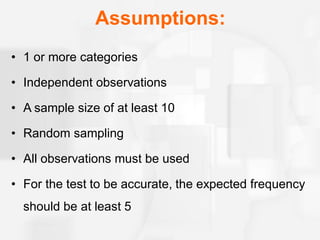
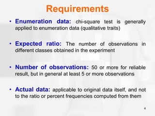
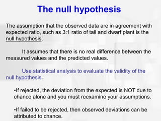
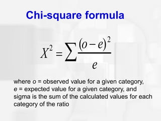
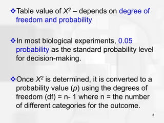
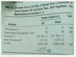
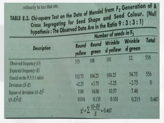
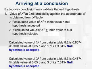
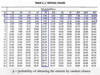
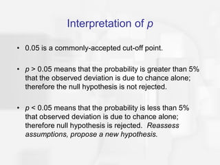
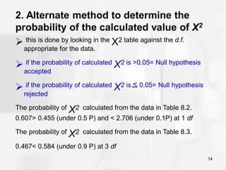
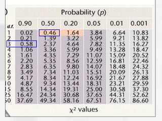
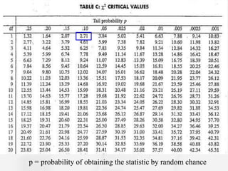
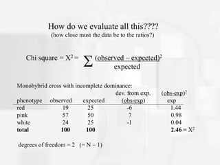
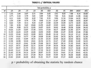
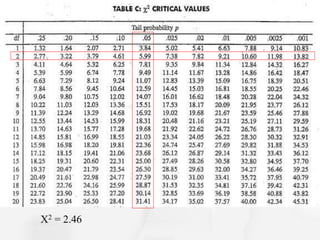
1
The Chi-Square Statistic
Dr. Prabhat Kr. Singh
Assistant Professor,
Department of Genetics and Plant Breeding
MSSSoA, CUTM, Paralakhemundi, Odisha, India
Purpose
• To measure discontinuous categorical/binned data in which
a number of subjects fall into categories
• We want to compare our observed data to what we expect
to see. Due to chance? Due to association?
• When can we use the Chi-Square Test?
– Testing outcome of Mendelian Crosses, Testing Independence – Is
one factor associated with another?, Testing a population for
expected proportions
Assumptions:
• 1 or more categories
• Independent observations
• A sample size of at least 10
• Random sampling
• All observations must be used
• For the test to be accurate, the expected frequency
should be at least 5
Requirements
• Enumeration data: chi-square test is generally
applied to enumeration data (qualitative traits)
• Expected ratio: The number of observations in
different classes obtained in the experiment
• Number of observations: 50 or more for reliable
result, but in general at least 5 or more observations
• Actual data: applicable to original data itself, and not
to the ratio or percent frequencies computed from them
4
The null hypothesis
The assumption that the observed data are in agreement with
expected ratio, such as 3:1 ratio of tall and dwarf plant is the
null hypothesis.
It assumes that there is no real difference between the
measured values and the predicted values.
Use statistical analysis to evaluate the validity of the
null hypothesis.
•If rejected, the deviation from the expected is NOT due to
chance alone and you must reexamine your assumptions.
•If failed to be rejected, then observed deviations can be
attributed to chance.
Chi-square formula
X2
=
(o− e)2
e

where o = observed value for a given category,
e = expected value for a given category, and
sigma is the sum of the calculated values for each
category of the ratio
Conducting Chi-Square Analysis
1) Make a null hypothesis based on your basic
biological question
2) Determine the expected frequencies
3) Create a table with observed frequencies,
expected frequencies, and chi-square values
using the X2 formula
4) Find the degrees of freedom: (n-1)
5) Find the chi-square statistic in the Chi-Square
Distribution table
6) Determine if null hypothesis is either (a) rejected
or (b) not rejected
❖Table value of X2 – depends on degree of
freedom and probability
❖In most biological experiments, 0.05
probability as the standard probability level
for decision-making.
❖Once X2 is determined, it is converted to a
probability value (p) using the degrees of
freedom (df) = n- 1 where n = the number
of different categories for the outcome.
8
11
Arriving at a conclusion
By two way conclusion may validate the null hypothesis
1. Value of X2 at 0.05 probability against the appropriate df
is obtained from X2 table
➢if calculated value of X2 < table value = null
hypothesis accepted
➢ if calculated value of X2 > table value = null
hypothesis rejected
Calculated value of X2 from data in table 8.2 is 0.607<
X2 table value at 0.05 p and 1 df i.e 3.841- Null
hypothesis accepted
Calculated value of X2 from data in table 8.3 is 0.467<
X2 table value at 0.05 p and 3 df i.e 7.815- Null
hypothesis accepted
p = probability of obtaining the statistic by random chance
Interpretation of p
• 0.05 is a commonly-accepted cut-off point.
• p > 0.05 means that the probability is greater than 5%
that the observed deviation is due to chance alone;
therefore the null hypothesis is not rejected.
• p < 0.05 means that the probability is less than 5%
that observed deviation is due to chance alone;
therefore null hypothesis is rejected. Reassess
assumptions, propose a new hypothesis.
2. Alternate method to determine the
probability of the calculated value of X2
➢ this is done by looking in the X2 table against the d.f.
appropriate for the data.
➢ if the probability of calculated X2 is >0.05= Null hypothesis
accepted
➢ if the probability of calculated X2 is < 0.05= Null hypothesis
rejected
The probability of X2 calculated from the data in Table 8.2.
0.607> 0.455 (under 0.5 P) and < 2.706 (under 0.1P) at 1 df
The probability of X2 calculated from the data in Table 8.3.
0.467< 0.584 (under 0.9 P) at 3 df
14
d.f.
p = probability of obtaining the statistic by random chance
How do we evaluate all this????
(how close must the data be to the ratios?)
Chi square = Χ2 = (observed – expected)2
expected
Monohybrid cross with incomplete dominance:
dev. from exp. (obs-exp)2
phenotype observed expected (obs-exp) exp
red 19 25 -6 1.44
pink 57 50 7 0.98
white 24 25 -1 0.04
total 100 100 2.46 = Χ2
degrees of freedom = 2 (= N – 1)
p = probability of obtaining the statistic by random chance
Χ2 = 2.46
Thank you

chi square statistics

  • 1.
    1 The Chi-Square Statistic Dr.Prabhat Kr. Singh Assistant Professor, Department of Genetics and Plant Breeding MSSSoA, CUTM, Paralakhemundi, Odisha, India
  • 2.
    Purpose • To measurediscontinuous categorical/binned data in which a number of subjects fall into categories • We want to compare our observed data to what we expect to see. Due to chance? Due to association? • When can we use the Chi-Square Test? – Testing outcome of Mendelian Crosses, Testing Independence – Is one factor associated with another?, Testing a population for expected proportions
  • 3.
    Assumptions: • 1 ormore categories • Independent observations • A sample size of at least 10 • Random sampling • All observations must be used • For the test to be accurate, the expected frequency should be at least 5
  • 4.
    Requirements • Enumeration data:chi-square test is generally applied to enumeration data (qualitative traits) • Expected ratio: The number of observations in different classes obtained in the experiment • Number of observations: 50 or more for reliable result, but in general at least 5 or more observations • Actual data: applicable to original data itself, and not to the ratio or percent frequencies computed from them 4
  • 5.
    The null hypothesis Theassumption that the observed data are in agreement with expected ratio, such as 3:1 ratio of tall and dwarf plant is the null hypothesis. It assumes that there is no real difference between the measured values and the predicted values. Use statistical analysis to evaluate the validity of the null hypothesis. •If rejected, the deviation from the expected is NOT due to chance alone and you must reexamine your assumptions. •If failed to be rejected, then observed deviations can be attributed to chance.
  • 6.
    Chi-square formula X2 = (o− e)2 e  whereo = observed value for a given category, e = expected value for a given category, and sigma is the sum of the calculated values for each category of the ratio
  • 7.
    Conducting Chi-Square Analysis 1)Make a null hypothesis based on your basic biological question 2) Determine the expected frequencies 3) Create a table with observed frequencies, expected frequencies, and chi-square values using the X2 formula 4) Find the degrees of freedom: (n-1) 5) Find the chi-square statistic in the Chi-Square Distribution table 6) Determine if null hypothesis is either (a) rejected or (b) not rejected
  • 8.
    ❖Table value ofX2 – depends on degree of freedom and probability ❖In most biological experiments, 0.05 probability as the standard probability level for decision-making. ❖Once X2 is determined, it is converted to a probability value (p) using the degrees of freedom (df) = n- 1 where n = the number of different categories for the outcome. 8
  • 11.
    11 Arriving at aconclusion By two way conclusion may validate the null hypothesis 1. Value of X2 at 0.05 probability against the appropriate df is obtained from X2 table ➢if calculated value of X2 < table value = null hypothesis accepted ➢ if calculated value of X2 > table value = null hypothesis rejected Calculated value of X2 from data in table 8.2 is 0.607< X2 table value at 0.05 p and 1 df i.e 3.841- Null hypothesis accepted Calculated value of X2 from data in table 8.3 is 0.467< X2 table value at 0.05 p and 3 df i.e 7.815- Null hypothesis accepted
  • 12.
    p = probabilityof obtaining the statistic by random chance
  • 13.
    Interpretation of p •0.05 is a commonly-accepted cut-off point. • p > 0.05 means that the probability is greater than 5% that the observed deviation is due to chance alone; therefore the null hypothesis is not rejected. • p < 0.05 means that the probability is less than 5% that observed deviation is due to chance alone; therefore null hypothesis is rejected. Reassess assumptions, propose a new hypothesis.
  • 14.
    2. Alternate methodto determine the probability of the calculated value of X2 ➢ this is done by looking in the X2 table against the d.f. appropriate for the data. ➢ if the probability of calculated X2 is >0.05= Null hypothesis accepted ➢ if the probability of calculated X2 is < 0.05= Null hypothesis rejected The probability of X2 calculated from the data in Table 8.2. 0.607> 0.455 (under 0.5 P) and < 2.706 (under 0.1P) at 1 df The probability of X2 calculated from the data in Table 8.3. 0.467< 0.584 (under 0.9 P) at 3 df 14
  • 15.
  • 16.
    p = probabilityof obtaining the statistic by random chance
  • 17.
    How do weevaluate all this???? (how close must the data be to the ratios?) Chi square = Χ2 = (observed – expected)2 expected Monohybrid cross with incomplete dominance: dev. from exp. (obs-exp)2 phenotype observed expected (obs-exp) exp red 19 25 -6 1.44 pink 57 50 7 0.98 white 24 25 -1 0.04 total 100 100 2.46 = Χ2 degrees of freedom = 2 (= N – 1)
  • 18.
    p = probabilityof obtaining the statistic by random chance
  • 19.
  • 20.