lecture 2.pdf

Fluid Mechanics II
ME-316
Fluid Kinematics
Dr. Syed Ahmad Raza
Department of Mechanical Engineering
NED University of Engineering & Technology
Karachi, Pakistan
Fall 2022

Fluid Mechanics II ME-316 (Fall 2022) Dr. Ahmad, Mechanical Engineering, NED UET, Pakistan
Objectives
At the end of this chapter, you should be able to do the following:
• Discuss the differences between the Eulerian and Lagrangian descriptions of fluid motion.
• Identify various flow characteristics based on the velocity field.
• Discuss various ways to visualize flow fields—streamlines, streaklines, pathlines, timelines,
optical methods schlieren and shadowgraph, and surface methods
• Determine the pattern of streamlines and acceleration field given a velocity field.
• Discuss the differences between a system and control volume.
• Apply the Reynolds transport theorem and the material derivative.
Fluid Kinematics 22110301 2

Outline
• Introduction
• Velocity field
• Acceleration field
• Control volume and system representation
• Reynolds transport theorem
• Examples
1Ref: https://www.flickr.com/photos/117994717@N06/34874208054/in/photostream/

Kinematics VS dynamics
The discipline of fluid mechanics is a discipline within the broad field of applied mechanics that is
concerned with the behavior of liquids and gases at rest or in motion.
Kinematics
It is the branch of mechanics dealing with the
study of the motion of a body or a system
of bodies without consideration given to its
mass or the forces acting on it.
Dynamics
It is the study of the motion of a body along
with the cause of motion, that is, the forces
and torques acting on the body.

Lagrangian description I
There are two distinct ways to describe motion. The first is to follow the path of individual objects.
For example, consider a ball on a pool table or a puck on an air hockey table colliding with another
ball or puck or with the wall. Newton’s laws are used to describe the motion of such objects, and we
can accurately predict where they go and how momentum and kinetic energy are exchanged from
one object to another. The kinematics of such experiments involves keeping track of the position
vector of each object, ®
xA, ®
xB, ...., and the velocity vector of each object, ®
VA, ®
VB......, as functions of
time. When this method is applied to a flowing fluid, we call it the Lagrangian description of fluid
motion.
Lagrangian analysis
The Lagrangian analysis is analogous to the closed system analysis of thermodynamics; namely,
we follow a mass of fixed identity. It involves following individual fluid particles as they move about
and determining how the fluid properties of these particles change as a function of time.

Lagrangian description II
The Lagrangian method of describing motion is much more difficult for fluids than for billiard balls.
First of all, we cannot easily define and identify fluid particles as they move around. Secondly, a fluid
is a continuum (from a macroscopic point of view), so interactions between fluid particles are not as
easy to describe as the interactions between distinct objects like billiard balls or air hockey pucks.
Furthermore, the fluid particles (each particle contains billions of molecules) continually deform
as they move in the flow. Nevertheless, there are many practical applications of the Lagrangian
description.
Practical applications
The tracking of passive scalars in a flow-to-model contaminant transport, rarefied gas dynamics
calculations concerning the reentry of a spaceship into the earth’s atmosphere, and the development
of flow visualization and measurement systems based on particle tracking.

Eulerian description
Out of the two distinct ways to describe fluid flow, a more common method is the Eulerian
description of fluid motion.
Instead of tracking individual fluid particles, we define field variables, functions of space and time,
within the control volume.
Eulerian analysis
In the Eulerian description of fluid flow, a finite volume called a flow domain or control volume is
defined, through which fluid flows in and out. The fluid motion is given by completely describing
the necessary properties as a function of space and time. We obtain information about the flow by
noting what happens at fixed points.

Examples for Lagrangian versus Eulerian descriptions
A river
Imagine a person standing
beside a river, measuring its
properties. In the
Lagrangian approach, he
throws in a probe that moves
downstream with the water.
In the Eulerian approach, he
anchors the probe at a fixed
location in the water.
A wind tunnel
In a wind tunnel, velocity or
pressure probes are usually
placed at fixed locations in
the flow, measuring the
respective V(x, y, z, t) or
P(x, y, z, t). This is an
Eulerian approach.
A bird
We may track the location of
a migrating bird using the
Lagrangian approach. Or
we may count birds passing a
particular location as per the
Eulerian description.
If you were going to study water flowing in a pipeline, which approach would you use? Eulerian.

Benefits of Lagrangian and Eulerian approaches for fluid mechanics studies
The advantage of Eulerian description
While there are many occasions in which the Lagrangian description is useful, the Eulerian de-
scription is often more convenient for applications of fluid mechanics. Furthermore, experimental
measurements are generally more suited to the Eulerian description.
The advantage of Lagrangian description
The equations of motion following an individual fluid particle are well known (e.g., Newton’s second
law) and can be written conveniently using the Lagrangian description. However, the equations of
motion of fluid flow are not so readily apparent in the Eulerian description and must be carefully
derived. We do this for control volume (integral) analysis via the Reynolds transport theorem
(RTT).
If we have enough information, we can obtain the Eulerian description from the Lagrangian descrip-
tion or vice versa.

Temperature measurement of a flowing fluid
Figure: Eulerian and Lagrangian descriptions of the temperature of a flowing fluid (figure 4.2).1
1Ref: Gerhart, P. M., Gerhart, A. L., Hochstein, J. I., Munson, B. R., Young, D. F., & Okiishi, T. H. (2016). Munson, young, and Okiishi’s fundamentals of Fluid Mechanics. Wiley.

Field variables
The field variable at a particular location at a particular time is the value of the variable for whichever
fluid particle happens to occupy that location at that time. For example, the pressure field is a scalar
field variable, whereas the velocity field is a vector field variable.
Common field variables for fluid flow
Pressure field: P = P(x, y, z, t)
Velocity field: V = V(x, y, z, t)
Acceleration field: a = a(x, y, z, t)
Collectively, these and other field variables define the flow field. The velocity field can be expanded
in Cartesian coordinates as
V = (u, v, w) = u(x, y, z, t)î + v(x, y, z, t)ĵ + w(x, y, z, t)k̂

12
FLOW PATTERNS AND FLOW VISUALIZATION
Spinning baseball. The late F. N. M.
Brown devoted many years to developing
and using smoke visualization in wind
tunnels at the University of Notre Dame.
Here the flow speed is about 23 m/s and
the ball is rotated at 630 rpm.
• Flow visualization: The visual
examination of flow field
features.
• While quantitative study of fluid
dynamics requires advanced
mathematics, much can be
learned from flow visualization.
• Flow visualization is useful not
only in physical experiments but
in numerical solutions as well
[computational fluid
dynamics (CFD)].
• In fact, the very first thing an
engineer using CFD does after
obtaining a numerical solution is
simulate some form of flow
visualization, so that he or she
can see the whole picture rather
than merely a list of numbers
and quantitative data.

Flow Patterns
 Fluid mechanics is a highly visual subject. The patterns of flow
can be visualized in a dozen different ways, and you can view
these sketches or photographs and learn a great deal
qualitatively and often quantitatively about the flow.
 Four basic types of line patterns are used to visualize flows:
1. Astreamline is a line everywhere tangent to the velocity
vector at a given instant.
2. Apathline is the actual path traversed by a given fluid
particle.
3. Astreakline is the locus of particles that have earlier passed
through a prescribed point.
4. Atimeline is a set of fluid particles that form a line at a
given instant.
13

14
Streamlines and Streamtubes
Streamline: A curve that is everywhere tangent to the instantaneous local
velocity vector.
Streamlines are useful as indicators of the instantaneous direction of fluid
motion throughout the flow field.
For example, regions of recirculating flow and separation of a fluid off of a
solid wall are easily identified by the streamline pattern.
Streamlines cannot be directly observed experimentally except in steady
flow fields.
Streamlines around a Nascar

15
A streamtube consists of a bundle
of individual streamlines.
In an incompressible flow field, a streamtube
(a) decreases in diameter as the flow
accelerates or converges and (b) increases in
diameter as the flow decelerates or diverges.
A streamtube consists of a bundle of
streamlines much like a
communications cable consists of a
bundle of fiber-optic cables.
Since streamlines are everywhere
parallel to the local velocity, fluid
cannot cross a streamline by
definition.
Fluid within a streamtube must
remain there and cannot cross the
boundary of the streamtube.
Both streamlines and
streamtubes are
instantaneous
quantities, defined at
a particular instant in
time according to the
velocity field at that
instant.

16
A streamline is a line that is everywhere tangent to
the velocity field.
Streamlines are obtained analytically by integrating
the equations defining lines tangent to the velocity
field. As illustrated in the figure, for two‐dimensional
flows the slope of the streamline, dy/dx, must be
equal to the tangent of the angle that the velocity
vector makes with the x axis or
𝑑𝑦
𝑑𝑥
𝑣
𝑢
If the velocity field is known as a function of x and y (and t if the flow is unsteady), this
equation can be integrated to give the equation of the streamlines.

17
Pathlines
• Pathline: The actual path
traveled by an individual fluid
particle over some time period.
• A pathline is a Lagrangian
concept in that we simply follow
the path of an individual fluid
particle as it moves around in
the flow field.
• Thus, a pathline is the same as
the fluid particle’s material
position vector (xparticle(t),
yparticle(t), zparticle(t)) traced out
over some finite time interval.
A pathline is formed by following the actual
path of a fluid particle.
Pathlines produced by white tracer particles suspended in
water and captured by time-exposure photography; as
waves pass horizontally, each particle moves in an elliptical
path during one wave period.
Particle image velocimetry (PIV): A modern experimental technique that
utilizes short segments of particle pathlines to measure the velocity field over
an entire plane in a flow.

18
Streaklines
Streakline: The locus of fluid
particles that have passed
sequentially through a
prescribed point in the flow.
Streaklines are the most
common flow pattern
generated in a physical
experiment.
If you insert a small tube into
a flow and introduce a
continuous stream of tracer
fluid (dye in a water flow or
smoke in an air flow), the
observed pattern is a
streakline. A streakline is formed by continuous
introduction of dye or smoke from a point in
the flow. Labeled tracer particles (1 through
8) were introduced sequentially.

19
Streaklines produced by
colored fluid introduced
upstream; since the flow is
steady, these streaklines are
the same as streamlines and
pathlines.
• Streaklines, streamlines, and pathlines are identical in steady flow
but they can be quite different in unsteady flow.
• The main difference is that a streamline represents an instantaneous
flow pattern at a given instant in time, while a streakline and a
pathline are flow patterns that have some age and thus a time history
associated with them.
• A streakline is an instantaneous snapshot of a time-integrated flow
pattern.
• A pathline, on the other hand, is the time-exposed flow path of an
individual particle over some time period.

21
Timelines
Timeline: A set of adjacent fluid particles
that were marked at the same (earlier)
instant in time.
Timelines are particularly useful in
situations where the uniformity of a flow
(or lack thereof) is to be examined.
Timelines are formed
by marking a line of
fluid particles, and
then watching that line
move (and deform)
through the flow field;
timelines are shown at
t = 0, t1, t2, and t3.
Timelines produced by a hydrogen bubble wire are used to visualize the
boundary layer velocity profile shape. Flow is from left to right, and the
hydrogen bubble wire is located to the left of the field of view. Bubbles near
the wall reveal a flow instability that leads to turbulence.

Comparisons
• For steady flow, streamlines, pathlines, and
streaklines are identical.
• For unsteady flow, they can be very different.
– Streamlines are an instantaneous picture of the flow field
– Pathlines and Streaklines are flow patterns that have a
time history associated with them.
– Streakline: instantaneous snapshot of a time‐integrated
flow pattern.
– Pathline: time‐exposed flow path of an individual particle.
22

Comparison of flow patterns in an unsteady flow
An unsteady, incompressible, two-dimensional velocity field is
given by
V = (u, v) = (0.5 + 0.8x)î + (1.5 + 2.5 sin(𝜔t) − 0.8y)ĵ
where the angular frequency 𝜔 is 2𝜋 rad/s (a physical frequency
of 1 Hz). Physically, you may imagine a flow into a large bell
mouth inlet that is oscillating up and down at a frequency of 1
Hz.
Figure: Streamlines, pathlines, and streaklines for an oscillating
velocity field. The streaklines and pathlines are wavy because of their
integrated time history, but the streamlines are not wavy since they
represent an instantaneous snapshot of the velocity field (example 4-5;
figure 4-27).1
1Ref: Cengel, Y. A., & Cimbala, J. M. (2018). Fluid Mechanics: Fundamentals and Applications. McGraw-Hill Education.

26
Refractive Flow Visualization Techniques
Another category of flow visualization is based on the refractive property of light waves.
As you recall from your study of physics, the speed of light through one material may differ
somewhat from that in another material, or even in the same material if its density
changes. As light travels through one fluid into a fluid with a different index of refraction,
the light rays bend (they are refracted).
There are two primary flow visualization techniques that utilize the fact that the index of
refraction in air (or other gases) varies with density. They are the shadowgraph technique
and the schlieren technique
Schlieren
image of
natural
convection
due to a
barbeque
grill.
Color
schlieren
image of
Mach 3.0
flow from
left to
right over
a sphere.

Plots of Flow Data
• Flow data are the presentation of the flow properties
varying in time and/or space.
• A Profile plot indicates how the value of a scalar
property varies along some desired direction in the
flow field.
• A Vector plot is an array of arrows indicating the
magnitude and direction of a vector property at an
instant in time.
• A Contour plot shows curves of constant values of a
scalar property for the magnitude of a vector
property at an instant in time.
27

Profile plot
Profile plots of the horizontal component of velocity as a
function of vertical distance; flow in the boundary layer
growing along a horizontal flat plate.
28

Vector plot
Results of CFD calculations of flow
impinging on a block; (a) streamlines,
(b) velocity vector plot of the upper
half of the flow, and (c) velocity vector
plot, close‐up view revealing more
details in the separated flow region.

Contour plot
Contour plots of the pressure field due to flow impinging
on a block.
30

31
Types Of Fluid Flow:
1) One , Two & Three Dimensional Flows.
2) Steady & Unsteady Flows.
3) Uniform & Non‐uniform Flows.
4) Laminar & Turbulent Flows.
5) Compressible & Incompressible Flows.
6) Rotational & Irrotational Flows.

1D, 2D, and 3D Flows
Most fluid flows are complex three dimensional, time‐dependent phenomenon,
however we can make simplifying assumptions allowing an easier analysis or
understanding without sacrificing accuracy. In many cases we can treat the flow as 1D
or 2D flow.
Three‐Dimensional Flow: All three velocity components are important and of equal
magnitude. Flow past a wing is complex 3D flow, and simplifying by eliminating any
of the three velocities would lead to severe errors.
Two‐Dimensional Flow: In many situations one of the velocity components may
be small relative to the other two, thus it is reasonable in this case to assume 2D
flow.
One‐Dimensional Flow: In some situations two of the velocity components may be
small relative to the other one, thus it is reasonable in this case to assume 1D flow.
There are very few flows that are truly 1D, but there are a number where it is a
reasonable approximation.
32

33
Example: 2D – Flow Over An Airfoil
Longitudinal section of rectangular channel Cross-section V
elocity profile
velocity
Water surface
Example: 1D – Flow in an open channel

Steady flow:
It is the flow in which conditions of flow remains
constant w.r.t. time at a particular section but the
condition may be different at different sections.
Flow conditions: velocity, pressure, density or
cross‐sectional area etc.
e.g., A constant discharge through a pipe.
Unsteady flow :
It is the flow in which conditions of flow changes
w.r.t. time at a particular section.
e.g. A variable discharge through a pipe.
Steady and Unsteady flows
Steady –unsteady => Changing in time
34

Uniform flow:
The flow in which velocity at a given time does
not change with respect to space (length of
direction of flow) is called as uniform flow.
e.g. Constant discharge though a constant
diameter pipe.
Non – Uniform flow :
The flow in which velocity at a given time
changes with respect to space (length of
direction of flow) is called as non – uniform
flow.
e.g., Constant discharge through variable
diameter pipe.
Uniform and Non‐uniform flow
Uniform – nonuniform => Changing in space
35

Laminar and Turbulent flow
– Laminar flow
• fluid moves along smooth paths
• viscosity damps any tendency to
swirl or mix
– Turbulent flow
• fluid moves in very irregular paths
• efficient mixing
• velocity at a point fluctuates
36

Rotational & Irrotational Flow
Rotational Flows :‐
The flow in which fuid particle while flowing
along stream lines rotate about their own axis is
called as rotational flow.
Irrotational Flows:‐
The flow in which the fluid particle while
flowing along stream lines do not rotate about
their axis is called as irrotational flow.
37

Flow Combinations
T
ype Example
Flow at constant rate through a duct of
uniform cross-section
Flow at constant rate through a duct of
non-uniform cross-section (tapering pipe)
Flow at varying rates through a long
straight pipe of uniform cross-section.
Flow at varying rates through a duct of
non-uniform cross-section.
1.Steady Uniform flow
2.Steady non-uniform
flow
3.Unsteady Uniform flow
4.Unsteady non-uniform
flow
38

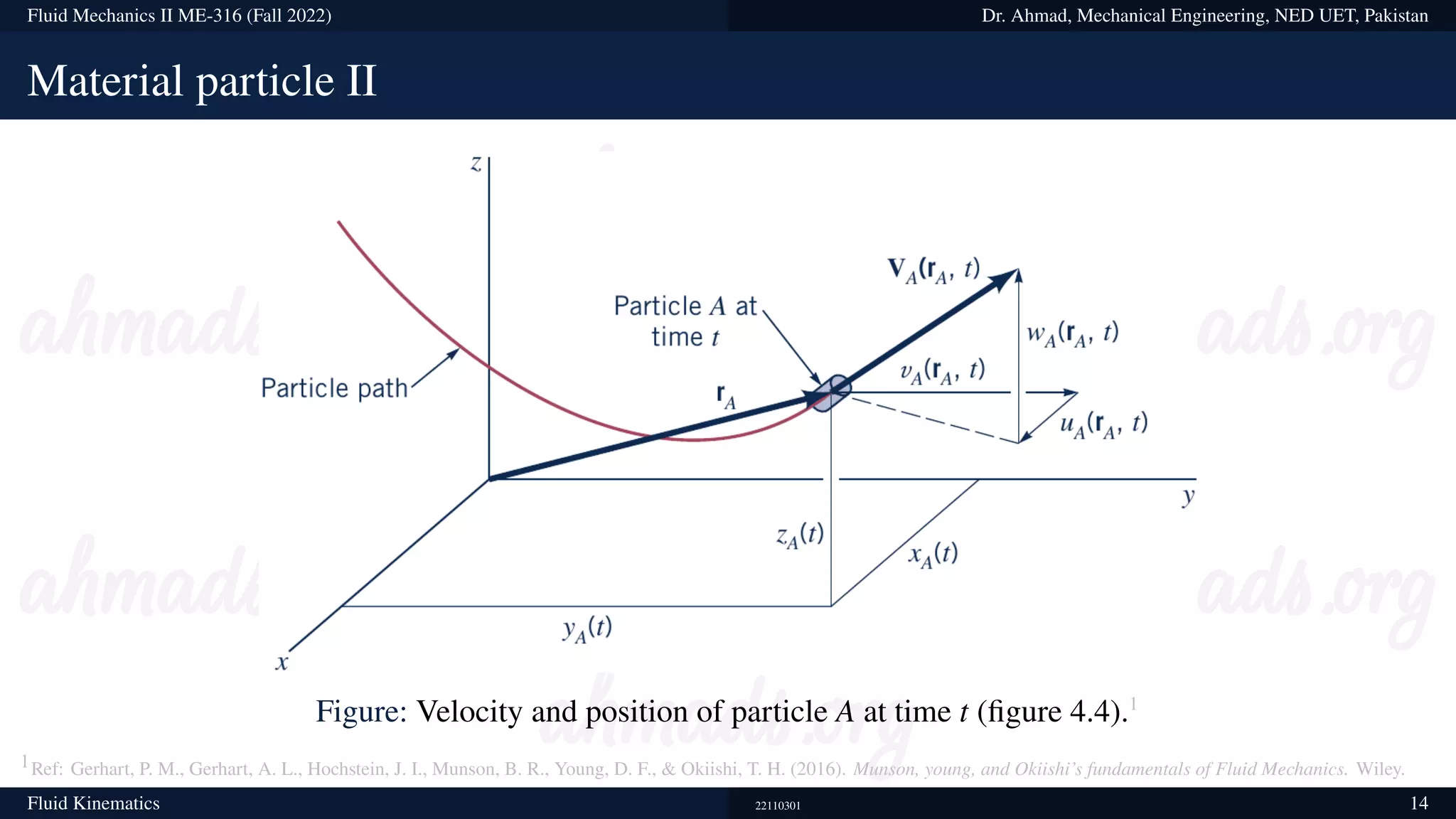
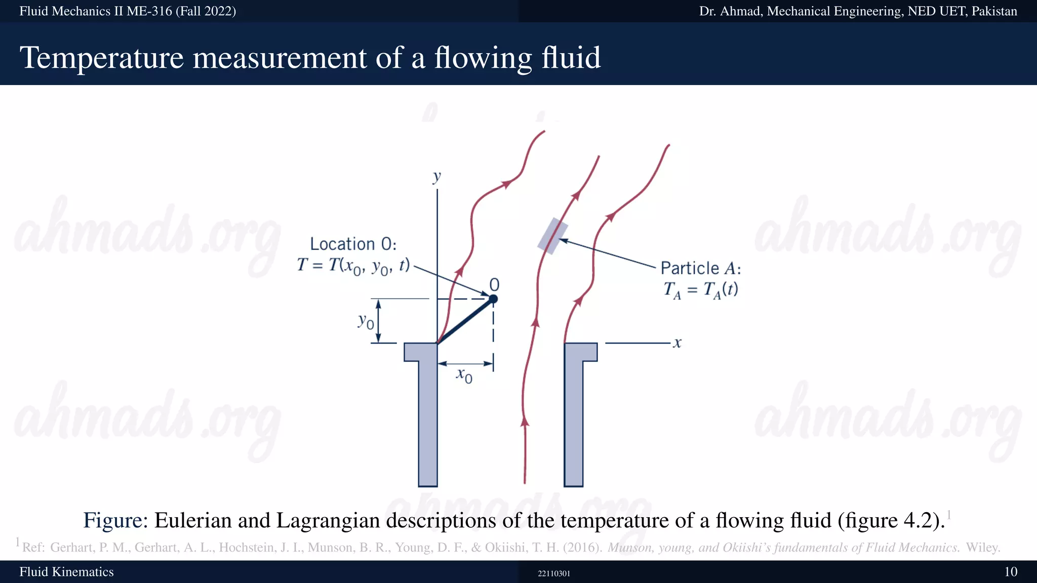
Material particle I
The equations of motion for fluid flow (such as Newton’s second law) can be written for a fluid
particle, which we also call a material particle. If we were to follow a particular fluid particle,
particle A, as it moves around in the flow, we would be employing the Lagrangian description, and
the equations of motion would be directly applicable. For example, we would define the particle A’s
location in space in terms of a material position vector,
rA = rA(t) = xA(t)î + yA(t)ĵ + zA(t)k̂ .
Similarly, the velocity vector for the particle A would be defined as
VA = VA(rA, t) = VA[(xA, t), (yA, t), (zA, t)] .
However, some mathematical manipulation is then necessary to convert the equations of motion into
forms applicable to the Eulerian description.

Material particle II
Figure: Velocity and position of particle A at time t (figure 4.4).1

Acceleration field and the material derivative
Consider Newton’s second law applied to the fluid particle A,
FA = mAaA
where FA is the net force acting on the particle, mA is the mass of
the particle, and aA is the acceleration of the fluid particle.
By definition, the acceleration of the fluid is the time derivative
of the fluid particle’s velocity,
aA =
dVA
dt
However, at any instant in time t, the velocity of the particle is
the same as the local value of the velocity field at the location,
VA = V(x, y, z, t)
The velocity components are functions of both space and time,
V(x, y, z, t) = u(x, y, z, t)î + v(x, y, z, t)ĵ + w(x, y, z, t)k̂
Ref: Gerhart, P. M., Gerhart, A. L., Hochstein, J. I.,
Munson, B. R., Young, D. F., & Okiishi, T. H. (2016).
Munson, young, and Okiishi’s fundamentals of Fluid
Mechanics. Wiley.

Chain rule applied to the acceleration
The acceleration of the fluid particle in x-
direction is given by,
ax =
du
dt
Since the dependent variable, u is a function of
four independent variables, therefore, we must
use the chain rule for the differentiation of a
multivariable function,
ax =
du
dt
=
du(x, y, z, t)
dt
ax =
𝜕u
𝜕x
dx
dt
+
𝜕u
𝜕y
dy
dt
+
𝜕u
𝜕z
dz
dt
+
𝜕u
𝜕t
dt
dt
where 𝜕 is the partial derivative operator and d
is the total derivative operator.
∵
dx
dt
= u,
dy
dt
= v, and
dz
dt
= w
ax = u
𝜕u
𝜕x
+ v
𝜕u
𝜕y
+ w
𝜕u
𝜕z
+
𝜕u
𝜕t
Similarly, for the y- and z-components, we obtain
ay = u
𝜕v
𝜕x
+ v
𝜕v
𝜕y
+ w
𝜕v
𝜕z
+
𝜕v
𝜕t
az = u
𝜕w
𝜕x
+ v
𝜕w
𝜕y
+ w
𝜕w
𝜕z
+
𝜕w
𝜕t
At any instant in time t, the acceleration field
(a = a(x, y, z, t)) must equal the acceleration of
the fluid particle that happens to occupy the lo-
cation (x, y, z) it is accelerating with the fluid
flow. Hence, the above acceleration may be in-
terpreted in the Eulerian frame of reference.

45
Material Derivative ‐‐‐‐ Acceleration Field (continued)
The total derivative operator d/dt in Eq. above is given a special name, the material
derivative; it is assigned a special notation, D/Dt, in order to emphasize that it is formed by
following a fluid particle as it moves through the flow field. Other names for the material
derivative include total, particle, Lagrangian, Eulerian, and substantial derivative.
Material derivative: 𝐃
𝐃𝐭
𝐝
𝐝𝐭
𝛛
𝛛𝐭
𝐕. 𝛁
When we apply the material derivative of Eq. to the velocity field, the result is the
acceleration field as expressed by following Eq, which is thus sometimes called the material
acceleration,
Material acceleration: 𝑎
⃗ 𝑥, 𝑦, 𝑧, 𝑡
𝐷𝑉
𝐷𝑡
𝑑𝑉
𝑑𝑡
𝜕𝑉
𝜕𝑡
𝑉. 𝛻 𝑉
For example, the material derivative of pressure is written as
Material derivative of pressure:
V. 𝛻 T u v w
Material derivative of temperature:
DP
Dt
dP
dt
𝜕P
𝜕t
V. 𝛻 P
u v w

44
Material Derivative ‐‐‐‐ Acceleration Field (continued)
Inspection of above equations reveal that the terms on the right hand sides are of two
different types: those that include changes of velocity with respect to position , 𝑢 ,
𝑣 , and so on; and those that are changes of velocity with respect to time , , and
.
Terms of the first type are called CONVECTIVE acceleration because they are
associated with velocity changes that occur because of changes in position in the flow
field.
However, the second type, acceleration results because the velocity changes with
respect to time at a given point. These are called LOCAL acceleration.
Obviously, local acceleration results when the flow is unsteady and convective
acceleration occurs when the flow is no‐uniform, that is when velocity changes along a
stream line.

46
Unsteady Effects
If a flow is unsteady, its parameter values (velocity, temperature, density, etc.) at any
location may change with time. For example, an unstirred (v=0) cup of coffee will cool
down in time because of heat transfer to its surroundings.
V. 𝛻 T u v w
DT
Dt
𝜕T
𝜕t
Consider flow in a constant diameter pipe as is shown in Fig. The flow is assumed
to be spatially uniform throughout the pipe. That is, at all points in the pipe. The
acceleration field may vary with time.
𝑎
⃗ 𝑥, 𝑦, 𝑧, 𝑡
𝐷𝑉
𝐷𝑡
𝑑𝑉
𝑑𝑡
𝜕𝑉
𝜕𝑡
𝑉. 𝛻 𝑉
𝑎
⃗ 𝑥, 𝑦, 𝑧, 𝑡
𝐷𝑉
𝐷𝑡
𝜕𝑉
𝜕𝑡
0
0 0 0

47
Convective Effects
The temperature of a water particle changes as it flows through
a water heater. The water entering the heater is always the
same cold temperature, and the water leaving the heater is
always the same hot temperature. The flow is steady. However,
the temperature, T, of each water particle increases as it passes
through the heater
u v w
V. 𝛻 T u v w
The portion of the material derivative represented by the spatial
derivatives is termed the convective derivative. It represents
the fact that a flow property associated with a fluid particle may
vary because of the motion of the particle from one point in
space where the
parameter has one value to another point in space where its
value is different. For example, the water velocity at the inlet of
the garden hose nozzle shown in the figure is different (both in
direction and speed) than it is at the exit. This contribution to the
time rate of change of the parameter for the particle can occur
whether the flow is steady or unsteady.

48
The same types of processes are involved with fluid accelerations. Consider flow in a
variable area pipe as shown in Fig. It is assumed that the flow is steady and one‐dimensional
with velocity that increases and decreases in the flow direction as indicated.

53
Streamline Coordinates
In many flow situations, it is convenient to use a coordinate system defined in terms of the
streamlines of the flow.
In the streamline coordinate system the flow is described in terms of one coordinate
along the streamlines, denoted s, and the second coordinate normal to the streamlines,
denoted n.

54
Unit vectors in these two directions are denoted by 𝑠̂ and 𝑛 as shown in the figure
Care is needed not to confuse the coordinate distance s (a scalar) with the unit
vector along the streamline direction, 𝑠̂.

56
Control Volume and System Representations
In thermodynamics and solid mechanics we often work with a system (also called a closed
system), defined as a quantity of matter of fixed identity. In fluid dynamics, it is more common
to work with a control volume (also called an open system), defined as a region in space
chosen for study. The size and shape of a system may change during a process, but no mass
crosses its boundaries. A control volume, on the other hand, allows mass to flow in or out
across its boundaries, which are called the control surface. A control volume may also move
and deform during a process, but many real‐world applications involve fixed, nondeformable
control volumes.
Two methods of analyzing the spraying
of deodorant from a spray can:
(a)We follow the fluid as it moves and deforms.
This is the system approach—no mass crosses
the boundary, and the total mass of the system
remains fixed.
(b)We consider a fixed interior volume of the can.
This is the control volume approach—
mass crosses the boundary
As with any matter, a fluid’s behavior is governed by fundamental physical laws that are
approximated by an appropriate set of equations. The application of laws such as the
conservation of mass, Newton’s laws of motion, and the laws of thermodynamics forms the
foundation of fluid mechanics analyses. There are various ways that these governing laws can
be applied to a fluid, including the system approach and the control volume approach.

Control Volume and System Representations
Fixed Control Volume:
Fixed or Moving
Control Volume:
Deforming Control
Volume:
Surface of the Pipe
Surface of the Fluid
Volume Around The Engine
Inflow
Outflow
Outflow Deforming Volume
Control Volume and System Representations (continued)
57

58
Most principles of fluid mechanics are adopted from solid mechanics, where the physical laws
dealing with the time rates of change of extensive properties are expressed for systems. In
fluid mechanics, it is usually more convenient to work with control volumes, and thus there is
a need to relate the changes in a control volume to the changes in a system. The relationship
between the time rates of change of an extensive property for a system and for
a control volume is expressed by the Reynolds transport theorem (RTT)
Control Volume and System Representations (continued)
The relationship between the time rates
of change of an extensive property for a
system and for a control volume is
expressed by the Reynolds transport
theorem (RTT).
The Reynolds transport theorem
(RTT) provides a link between
the system approach and the
control volume approach.

59
Mass Momentum Kinetic
Energy
Angular
momentum
B, Extensive properties m 𝑚𝑉
2
b, Intensive properties 1 𝑉
2
mV

V

Reynolds Transport Theorem
Preliminary Concepts
All the laws of governing the motion of a fluid are stated in their basic form in terms
of a system approach, and not in terms of a control volume.
The Reynolds Transport Theorem allows us to shift from the system approach to
the control volume approach, and back.
General Concepts:
B represents any of the fluid properties, m represent the mass, and b
represents the amount of the parameter per unit volume.
B is termed an extensive property, and b is an intensive property. B is
directly proportional to mass, and b is independent of mass.

Reynolds Transport Theorem: Preliminary Concepts
For a System: The amount of an extensive property can be calculated by adding
up the amount associated with each fluid particle.
Now, the time rate of change of that system:
Now, for control volume:
For the control volume, we only integrate over the control volume, this is
different integrating over the system, though there are instance when they
could be the same. 60

61
Reynolds Transport Theorem:
Derivation
A moving system (hatched region) and
a fixed control volume (shaded region)
in a diverging portion of a flow field at
times t and t+t. The upper and lower
bounds are streamlines of the flow.
The time rate of change of the
property B of the system is equal to
the time rate of change of B of the
control volume plus the net flux of B
out of the control volume by mass
crossing the control surface.
This equation applies at any instant
in time, where it is assumed that
the system and the control volume
occupy the same space at that
particular instant in time.

Reynolds transport theorem
Figure: Control volume and system for flow through a variable area pipe (figure 4.11).1

Consider a 1D flow through a fixed control volume between
(1) and (2). At time t, both the control volume and the system
(closed system) coincide. But at time t + 𝛿t, the system has
moved forward. The inflow into the control volume at time
t + 𝛿t is denoted as volume I, and the outflow as volume II.
The system boundary at the left-hand side moves forward by
𝛿l1 = V1𝛿t, while the system boundary at the right-hand side
moves forward by 𝛿l2 = V2𝛿t.
We may write the equation at both times in terms of the
extensive parameter:
Bsys(t) = Bcv(t)
Bsys(t + 𝛿t) = Bcv(t + 𝛿t) − BI(t + 𝛿t) + BII(t + 𝛿t) Ref: Gerhart, P. M., Gerhart, A. L., Hochstein, J. I., Munson, B.
R., Young, D. F., & Okiishi, T. H. (2016). Munson, young, and
Okiishi’s fundamentals of Fluid Mechanics. Wiley.

Bsys(t) = Bcv(t)
Bsys(t+𝛿t) = Bcv(t+𝛿t) − BI(t+𝛿t) + BII(t+𝛿t)
Subtracting the first equation from the second and dividing by
𝛿t throughout, we get
Bsys(t+𝛿t)−Bsys(t)
𝛿t
=
Bcv(t+𝛿t)−BI(t+𝛿t)+BII(t+𝛿t)−Bcv(t)
𝛿t
𝛿Bsys
𝛿t
|{z}
1
=
Bcv(t+𝛿t) − Bcv(t)
𝛿t
| {z }
2
−
BI(t+𝛿t)
𝛿t
| {z }
3
+
BII(t+𝛿t)
𝛿t
| {z }
4
Ref: Gerhart, P. M., Gerhart, A. L., Hochstein, J. I., Munson, B.
R., Young, D. F., & Okiishi, T. H. (2016). Munson, young, and
Okiishi’s fundamentals of Fluid Mechanics. Wiley.

Let 𝛿t → 0.
The time rate of change of B within the system:
1
𝛿Bsys
𝛿t
⇒
DBsys
Dt
The time rate of change of B within the control volume:
2
𝛿t
⇒ lim
𝛿t→0
𝛿t
=
𝜕Bcv
𝜕t
=
𝜕
∫
cv
𝜌bdV

𝜕t
The rate at which B flows into the control surface at (1) with 𝛿V1 = A1𝛿l1 = A1(V1𝛿t):
3
BI(t+𝛿t)
𝛿t
=
𝜌1b1𝛿V1
𝛿t
=
𝜌1b1A1V1𝛿t
𝛿t
⇒ lim
𝛿t→0
BI(t+𝛿t)
𝛿t
= ¤
Bin = 𝜌1A1V1b1
The rate at which B flows out of the control surface at (2) with 𝛿V2 = A2𝛿l2 = A2(V2𝛿t):
4
BII(t+𝛿t)
𝛿t
=
𝜌2b2𝛿V2
𝛿t
=
𝜌2b2A2V2𝛿t
𝛿t
⇒ lim
𝛿t→0
BII(t+𝛿t)
𝛿t
= ¤
Bout = 𝜌2A2V2b2

Therefore, by collecting all the terms, we get
DBsys
Dt
=
𝜕Bcv
𝜕t
+ ¤
Bout − ¤
Bin
DBsys
Dt
=
𝜕
𝜕t
∫
cv
𝜌bdV + 𝜌2A2V2b2 − 𝜌1A1V1b1
However, the following restrictions apply to this equation:
• Fixed control volume
• One inlet and one outlet
• Uniform properties (density, velocity, and the parameter b) across the inlet and outlet
• Velocity normal to sections (1) and (2)

Example 4.8
Problem
Consider the fluid flowing out of the fire extinguisher shown in
the figure. Let the extensive property of interest be the system
mass. Write the appropriate form of the Reynolds transport
theorem for this flow.
Solution
With B = m, the system mass, it follows that b = 1. We take the control volume to be the fire
extinguisher and the system to be the fluid within it at time t = 0. In this case, there is no inlet across
which the fluid flows into the control volume (Ain = 0) and using the basic law of conservation of
mass, the rate of change of mass in the system may be set to zero. Therefore, the Reynolds transport
theorem can be written as

0
Dmsys
Dt
=
𝜕
𝜕t
∫
cv
𝜌bdV + 𝜌outAoutVout ⇒
𝜕
𝜕t
∫
cv
𝜌bdV = − 𝜌outAoutVout
Ref: Gerhart, P. M., Gerhart, A. L., Hochstein, J. I., Munson, B. R., Young, D. F., Okiishi, T. H. (2016). Munson, young, and Okiishi’s fundamentals of Fluid Mechanics. Wiley.

Reynolds transport theorem for a CV with multiple inlets and outlets
In general, a control volume may contain more (or less) than one inlet and one outlet. A typical
pipe system may contain several inlets and outlets as shown in the figure below. In such instances,
we think of all the inlets summed together (I = Ia + Ib + Ic + ...) and all the outlets summed together
(II = IIa + IIb + IIc + ...), at least conceptually.
Figure: Typical control volume with more than one inlet and outlet (figure 4.13).1
1Ref: Gerhart, P. M., Gerhart, A. L., Hochstein, J. I., Munson, B. R., Young, D. F., Okiishi, T. H. (2016). Munson, young, and Okiishi’s fundamentals of Fluid Mechanics. Wiley.

Reynolds transport theorem for an arbitrary, fixed CV
A general, fixed control volume with fluid flow-
ing through it is shown in the figure. The
flow field may be quite simple (as in the pre-
vious one-dimensional flow considerations), or
it may involve a quite complex, unsteady, three-
dimensional situation such as the flow through a
human heart. In any case, we again consider the
system to be the fluid within the control volume
at the initial time t. A short time later a portion
of the fluid (region II) exited from the control
volume, and additional fluid (region I, not part of
the original system) entered the control volume.
Figure: Control volume and system for flow through
an arbitrary, fixed control volume (figure 4.12).1

Outflow and inflow across typical arbitrary, fixed control surfaces
Figure: Outflow across a typical portion of the control surface (figure 4.14).1
Figure: Inflow across a typical portion of the control surface (figure 4.15).1

Outflow and inflow across typical arbitrary, fixed control surfaces
For a general description, consider a differential
surface area dA on the control surface and denote
its unit outer normal by n̂. The flow rate of prop-
erty b through dA is (b𝜌V·n̂ dA) since the dot
product V·n̂ gives the normal component of the
velocity. Then the net rate of outflow through the
entire control surface is determined by integra-
tion to be ¤
Bnet = ¤
Bout − ¤
Bin =
∫
cs
b𝜌V·n̂ dA
where V·n̂ = |V||n̂| cos 𝜃 = V cos 𝜃 .
If 𝜃 90◦
, then cos 𝜃 0 i. e. outflow.
If 𝜃 90◦
, then cos 𝜃 0 i. e. inflow.
If 𝜃 = 90◦
, then cos 𝜃 = 0 i. e. no flow.

Reynolds transport theorem for an arbitrary, fixed control volume
RTT for an arbitrary, fixed control volume
DBsys
Dt
|{z}
1
=
𝜕
𝜕t
∫
cv
𝜌bdV
| {z }
2
+
∫
cs
b𝜌V·n̂ dA
| {z }
3
1 The time rate of change of the extensive parameter of a system such as mass, momentum, etc.
2 The time rate of change of the extensive parameter within the control volume.
3 The net flow rate of the extensive parameter across the entire control surface. The integral
∫
cs
b𝜌V·n̂ dA over the entire control surface gives the net amount of the property B flowing out of
the control volume (into the control volume of it is negative) per unit time. Note that 𝜌V·n̂ dA is
the net mass flow rate on a differential basis.

Reynolds Transport Theorem: Analogous to Material Derivative
Unsteady Portion Convective Portion
Steady Effects:
Unsteady Effects (inflow = outflow):
71
Steady flow through a control volume.
Unsteady flow through a constant
diameter pipe.

72
Relative velocity crossing a control surface is
found by vector addition of the absolute
velocity of the fluid and the negative of the
local velocity of the control surface.
Reynolds transport
theorem applied to a
control volume moving
at constant velocity.

73
Moving Control Volumes
It is the relative velocity CV
W V V
 
  
or CS
W V V
 
  
that carries the fluid
across the moving control surface.
ˆ
( )
sys
CV CS
DB d
bdV b W n dA
Dt dt
 
  
 

• Moving control volume - replace V with relative
velocity W = V-Vcv , where CV is moving at constant
velocity Vcv
• Deforming control volume – replace V with relative velocity
W + Vcs , where CS is moving at constant velocity Vcs

74
Conservation of Mass
ˆ
( )
sys
CV CS
DB d
bdV b V n dA
Dt dt
 
  
 

ˆ
1; 0 ( )
CV CS
Dm d
B m b dV V n dA
Dt dt
 
      
 

We know that , RTT is
Applying RTT for conservation of mass,
Steady flow:
ˆ
( ) 0
CS
V n dA
  



75
If the inlets and outlets are one‐dimensional the above equation simplifies to:
    0
i i i i i i
out in
i i
AV AV
 
 
 
Incompressible flow: ˆ
( ) 0
CS
V n dA
 


For the case of one‐dimensional inlets and outlets:     0
i i i i
out in
i i
AV AV
 
 
Equation of streamline:
In fluid mechanics the most common mathematical result for visualization purposes is
the streamline pattern. A typical set of streamlines and an arbitrary velocity vector is
shown in the figures below.
If the elemental arc length dr of a streamline is to be parallel to V, their respective
components must be in proportion: dx dy dz dr
u v w V
  

76
Relationship between Material Derivative and RTT
The Reynolds transport theorem for finite
volumes (integral analysis) is analogous to
the material derivative for infinitesimal
volumes (differential analysis). In both
cases, we transform from a Lagrangian or
system viewpoint to an Eulerian or control
volume viewpoint.
While the Reynolds transport
theorem deals with finite-size
control volumes and the
material derivative deals with
infinitesimal fluid particles, the
same fundamental physical
interpretation applies to both.
Just as the material derivative
can be applied to any fluid
property, scalar or vector, the
can be applied to any scalar or
vector property as well.

Reynolds—Transport Theorem (RTT)
There is a direct analogy between the transformation from
Lagrangian to Eulerian descriptions (for differential analysis using
infinitesimally small fluid elements) and the transformation from
systems to control volumes (for integral analysis using large,
finite flow fields).

78
Summary
• Lagrangian and Eulerian Descriptions
– Acceleration Field
– Material Derivative
• Flow Patterns and Flow Visualization
– Streamlines and Streamtubes, Pathlines,
– Streaklines, Timelines
– Refractive Flow Visualization Techniques
– Surface Flow Visualization Techniques
• Plots of Fluid Flow Data
– Profile Plots, Vector Plots, Contour Plots
• The Reynolds Transport Theorem
– Relationship between Material Derivative and RTT

lecture 2.pdf

Recommended

Recommended

More Related Content

What's hot

What's hot (20)

Similar to lecture 2.pdf

Similar to lecture 2.pdf (20)

Recently uploaded

Recently uploaded (20)

lecture 2.pdf