Download to read offline
![One row per process
• Each process starts with only one element of
x , need all-to-all broadcast to distribute all
the elements of x to all of the processes.
• Process Pi then computes
• The all-to-all broadcast and the computation
of y[i] both take time Θ(n) . Therefore, the
parallel time is Θ(n) .](https://image.slidesharecdn.com/densematrix-220723144848-66cb7dd9/75/densematrix-ppt-6-2048.jpg)
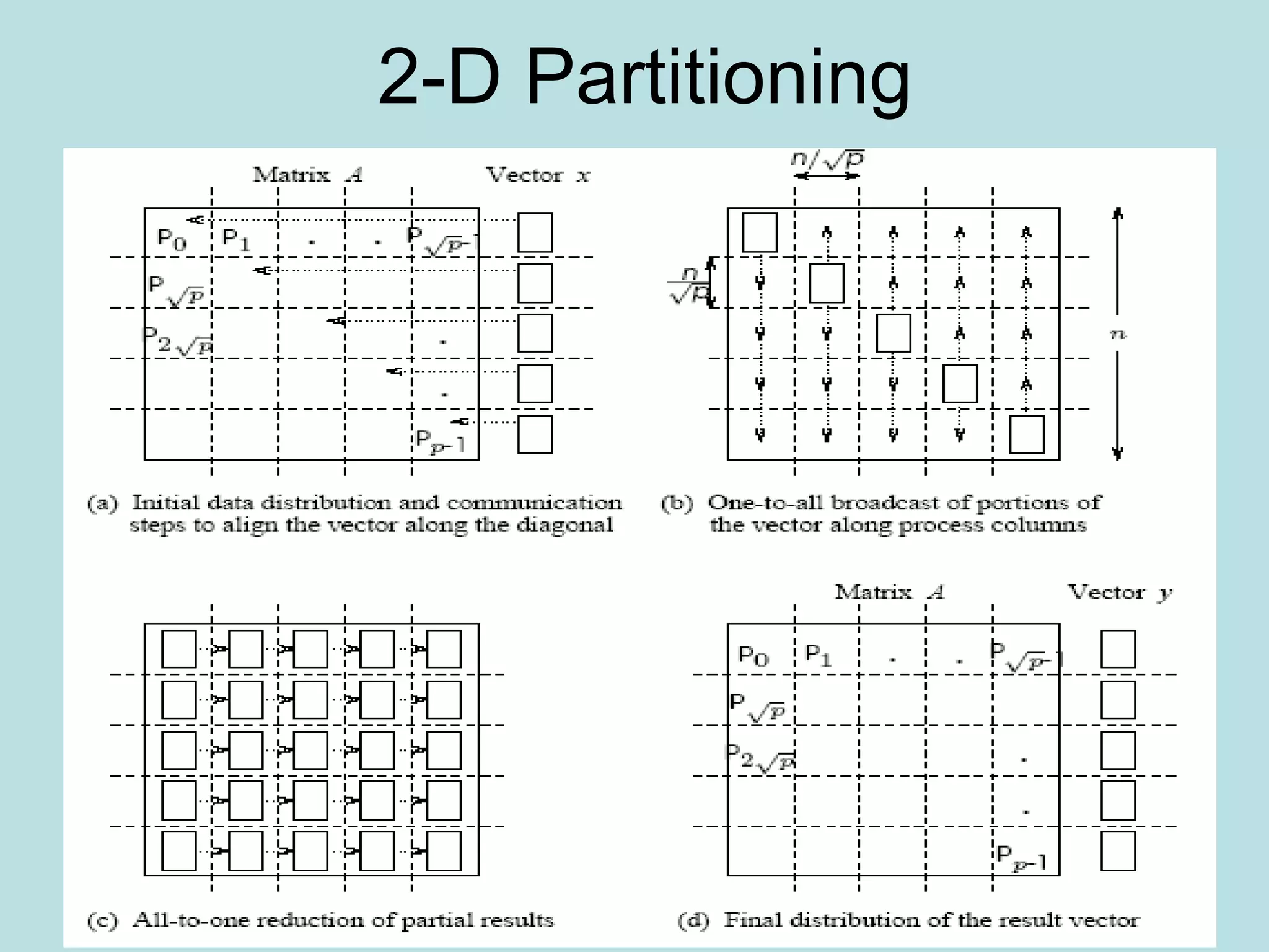
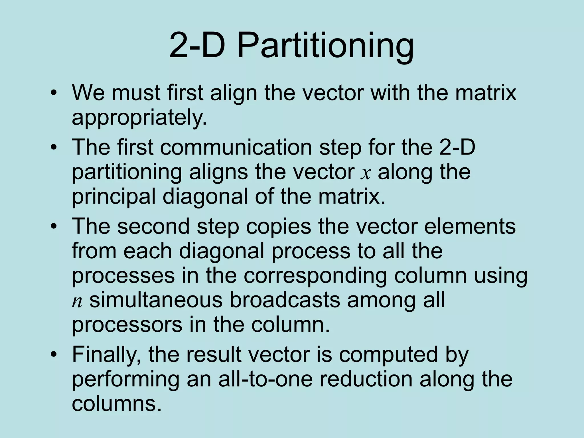


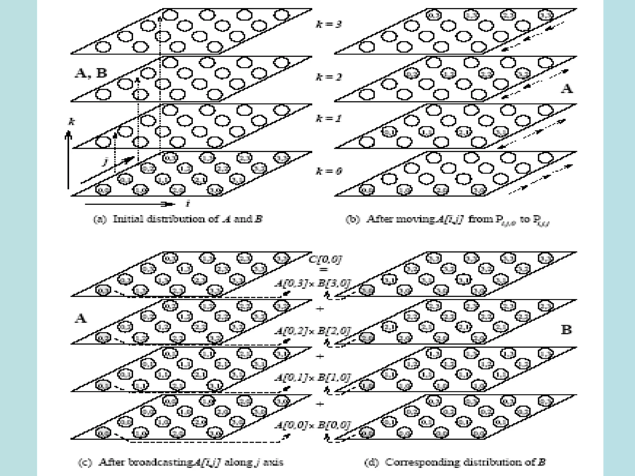


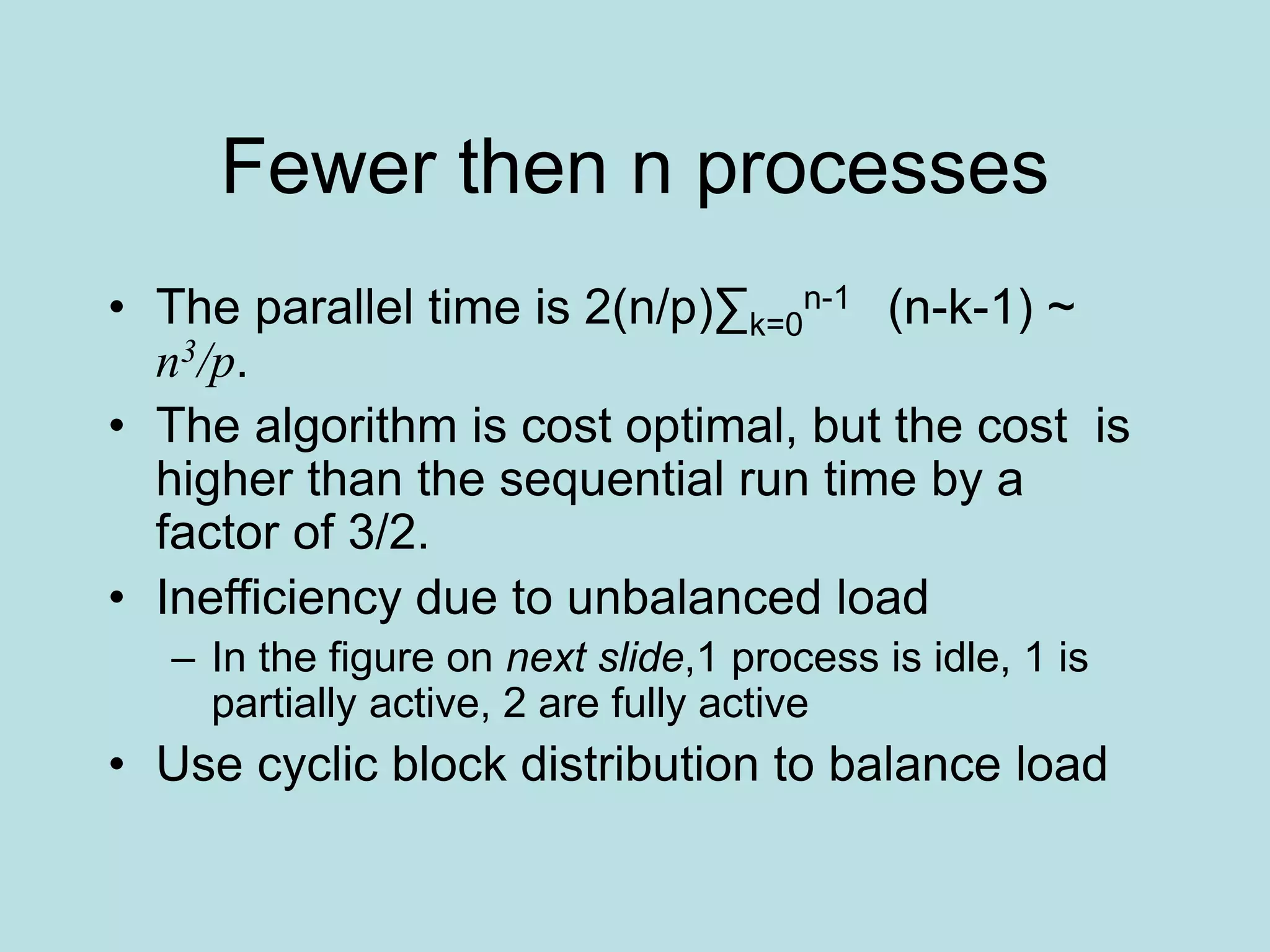
![2-D Partitioning
• A[i,j] is n x n and is mapped to n x n mesh-
A[i,j] goes to P I,J
• The rest is as before, only the communication
of individual elements takes place between
processors
• Need one to all broadcast of A[i,k] along ith
row for k≤ i<n and one to all broadcast of
A[k,j] along jth column for k<j<n
• Picture on next slide
• The result is not cost optimal](https://image.slidesharecdn.com/densematrix-220723144848-66cb7dd9/75/densematrix-ppt-48-2048.jpg)
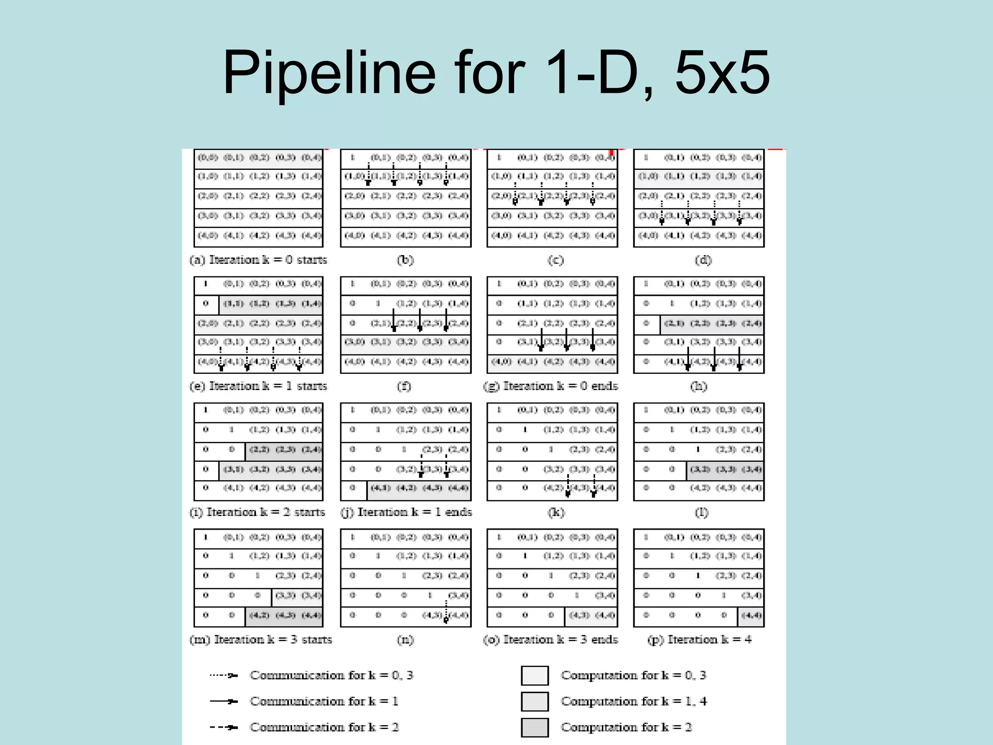
![Pipeline
• If we use synchronous broadcasts, the results
are not cost optimal, so we pipeline the 2-D
algorithm
• Principle of the pipelining algorithm is the
same-if you can compute or communicate, do
it now, not later
– P k,k+1 can divide A[k,k+1] by A[k,k] before A[k,k+1]
reaches P k,n-1 {the end of the row}
– After A[k,j] performs the division, it can send the
result down column j without waiting
• Next slide exhibits algorithm for 2-D pipelining](https://image.slidesharecdn.com/densematrix-220723144848-66cb7dd9/75/densematrix-ppt-50-2048.jpg)
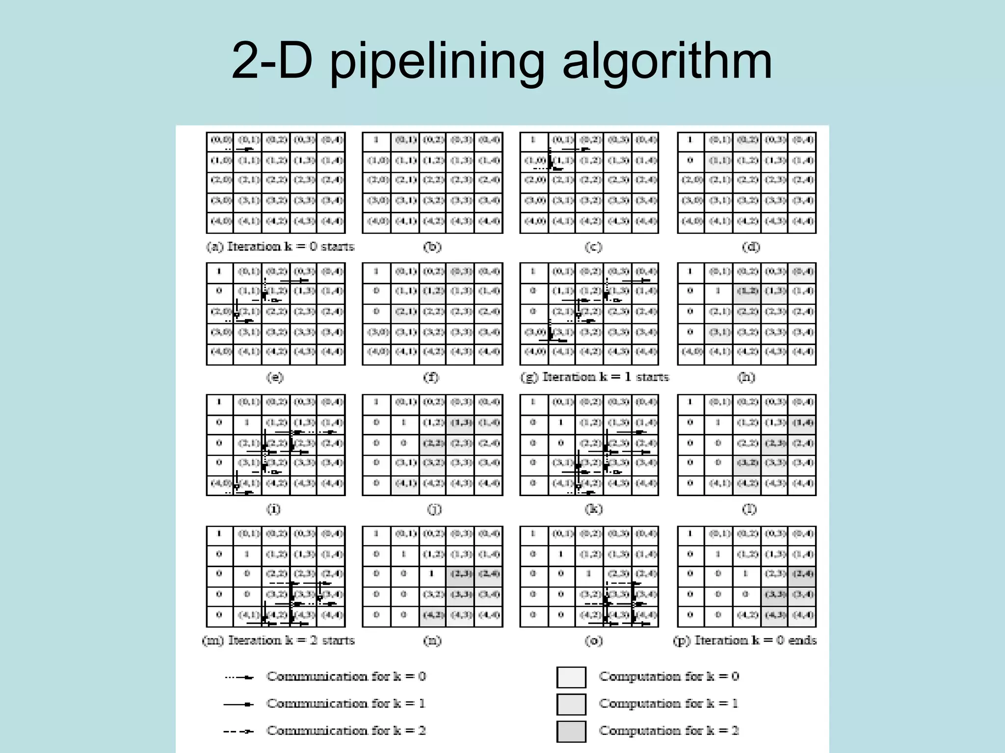
![Pipelining-the wave
• The computation and communication for each
iteration moves through the mesh from top-
left to bottom-right like a wave
• After the wave corresponding to a certain
iteration passes through a process, the
process is free to perform subsequent
iterations.
• In g, after k=0 wave passes P 1,1 it starts k=1 iteration by
passing A[1,1] to P 1,2.
• Multiple wave that correspond to different
iterations are active simultaneously.](https://image.slidesharecdn.com/densematrix-220723144848-66cb7dd9/75/densematrix-ppt-52-2048.jpg)


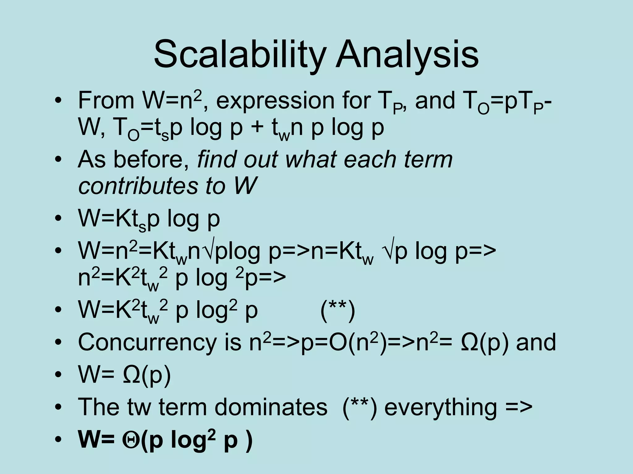
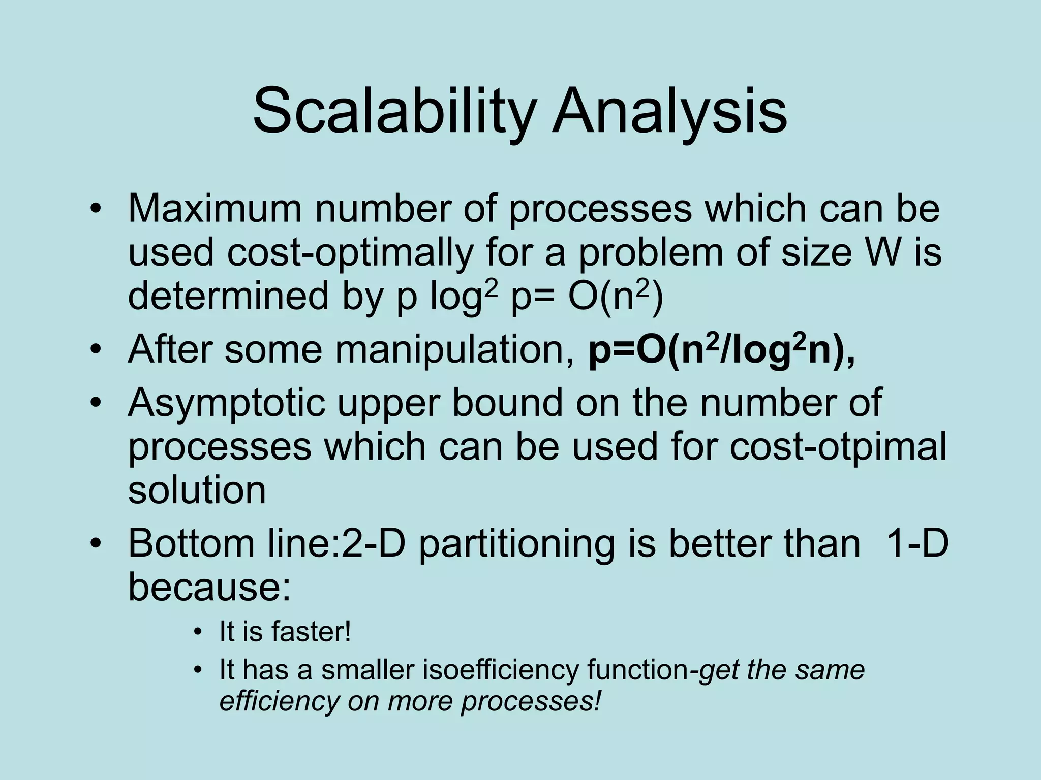
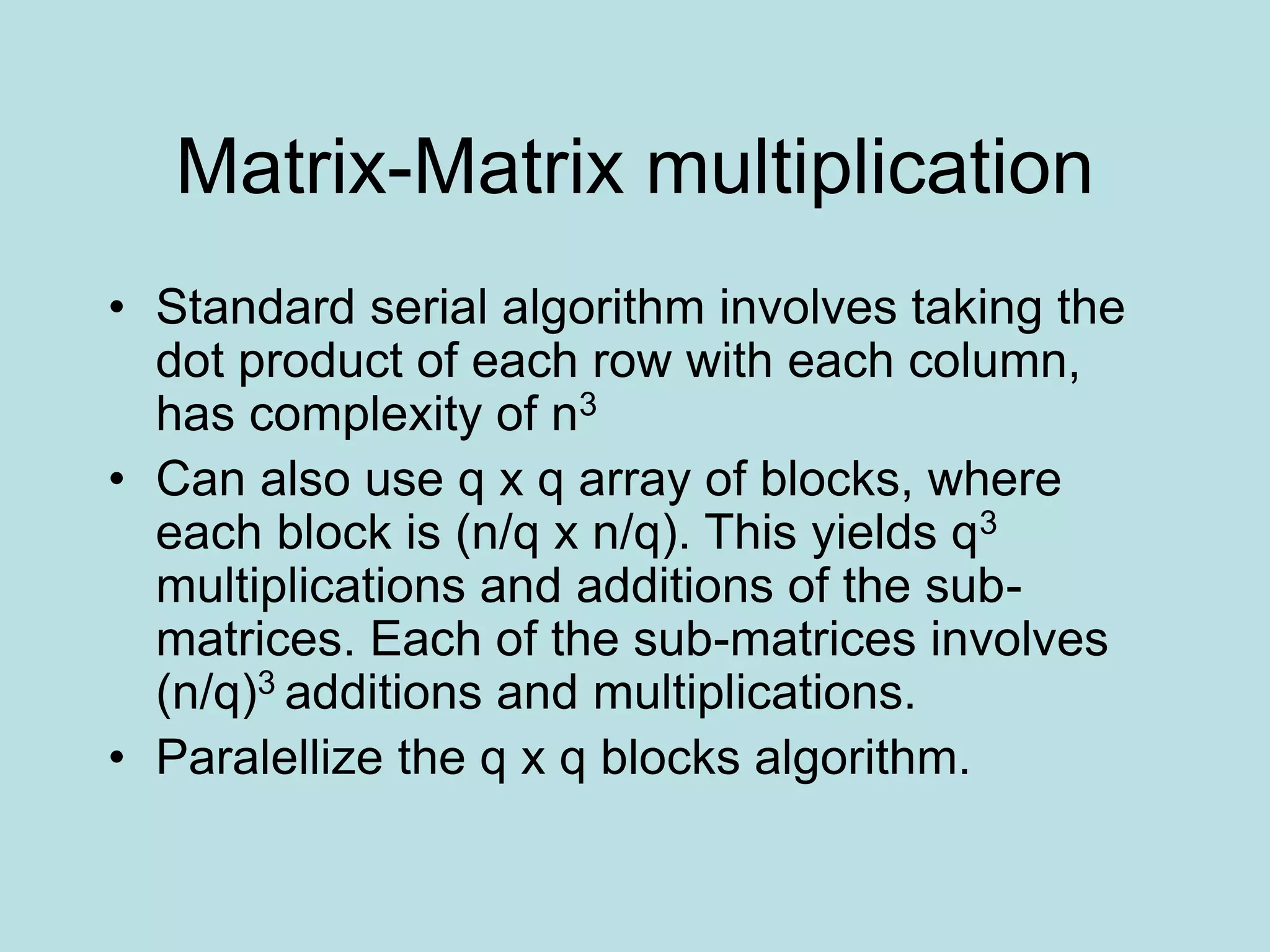
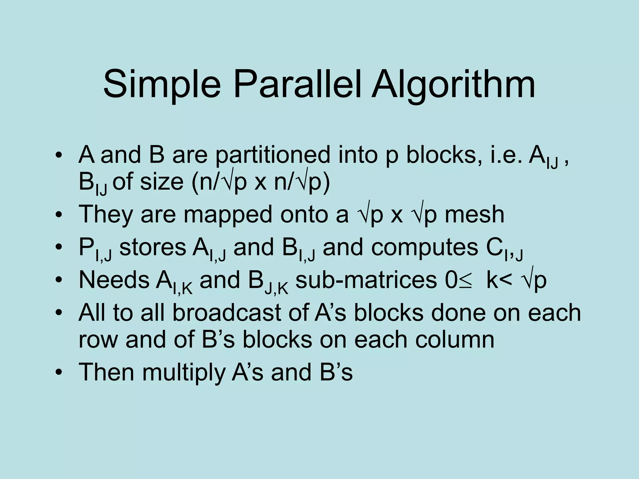
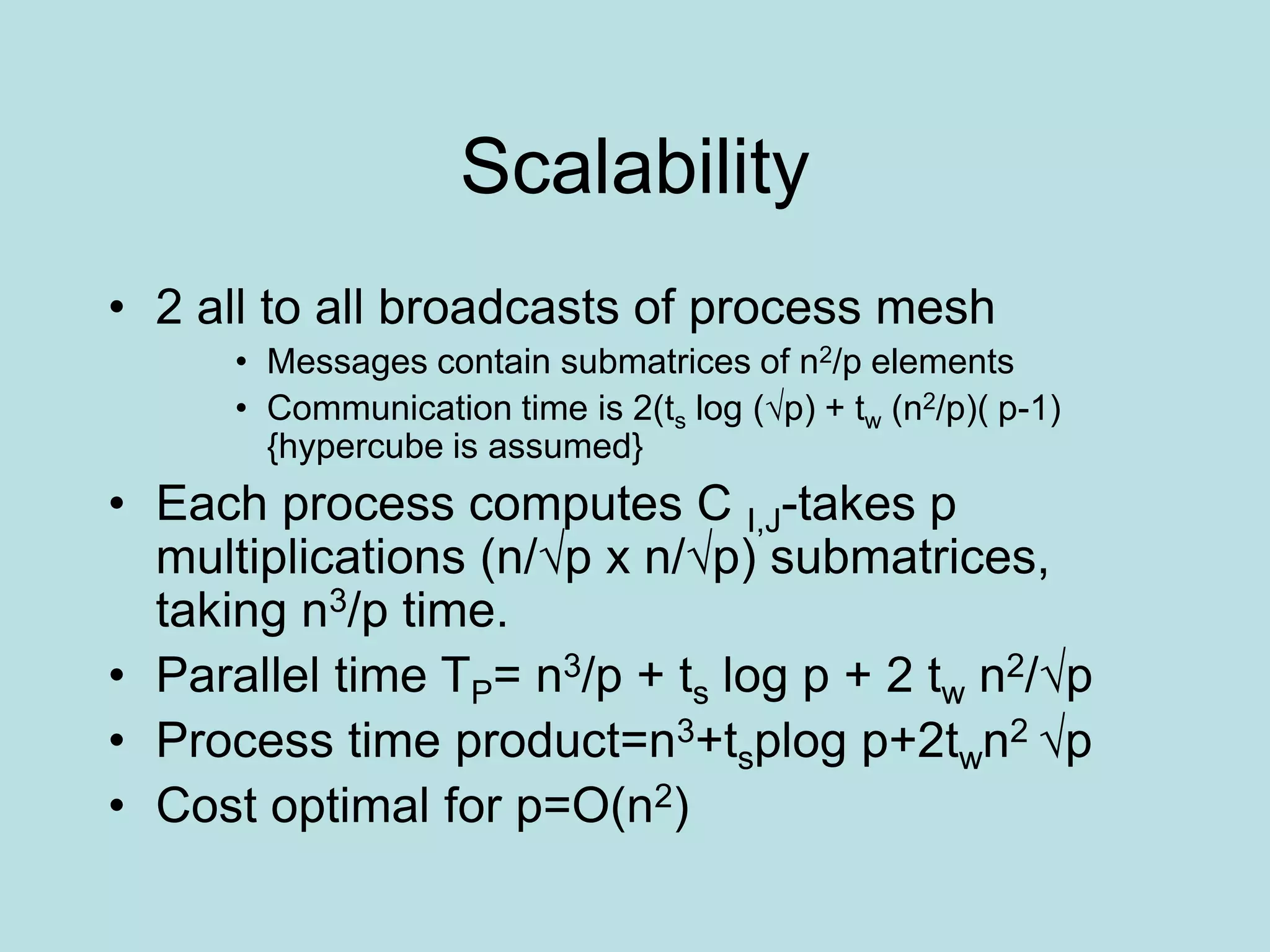
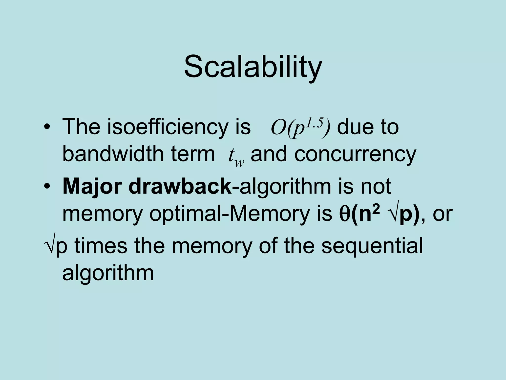
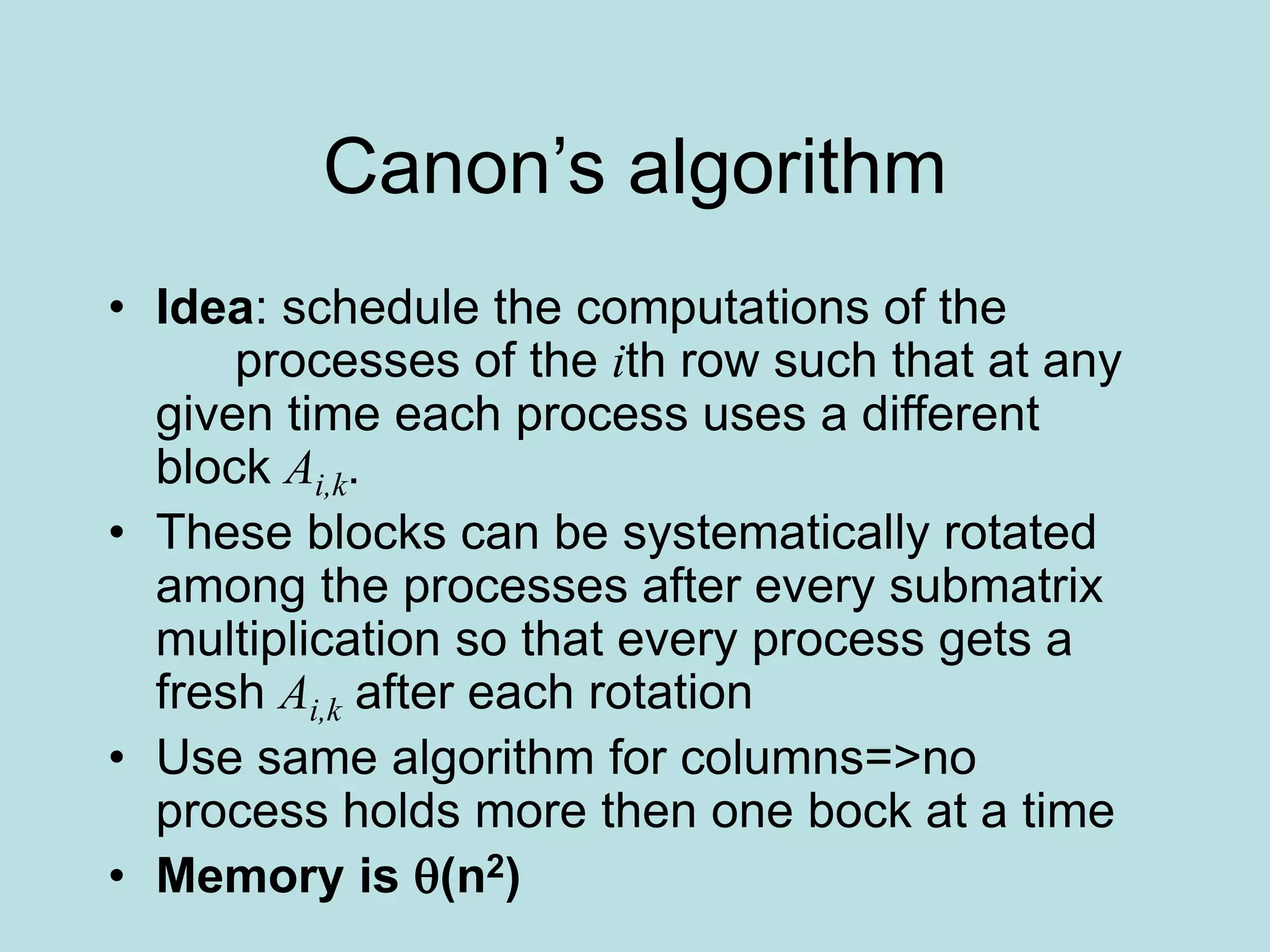
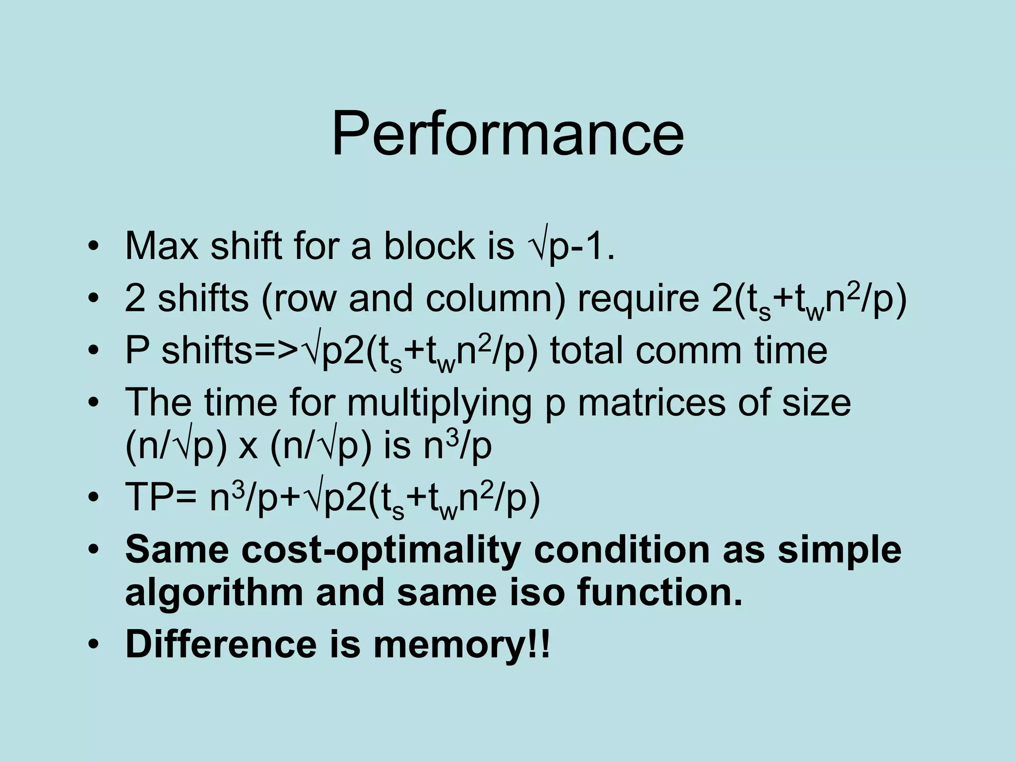
This document summarizes several dense matrix algorithms for operations like matrix-vector multiplication, matrix-matrix multiplication, and solving systems of linear equations. For matrix-vector multiplication, it describes 1D and 2D row-wise partitioning approaches. The 2D approach has lower parallel runtime of O(log n) but requires n2 processes. A modified 2D approach uses block partitioning and has parallel runtime of O(n/√p + log p) when using p < n2 processes. For matrix-matrix multiplication, simple parallel and Canon's algorithms are described. Canon's algorithm has optimal O(n3) memory usage by rotating matrix blocks among processes. A DNS algorithm achieves optimal O(log n