Standard deviation

1. Standard deviation
For other uses, see Standard Deviation (disambiguation).
In statistics, the standard deviation (SD) (represented
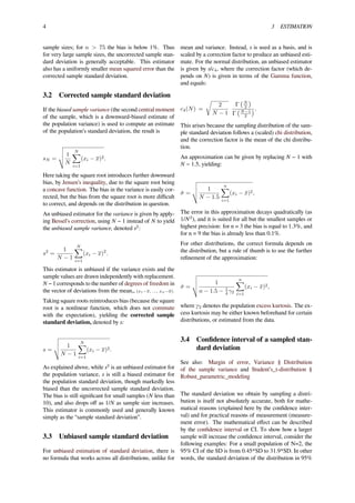
0.00.10.20.30.4
−2σ −1σ 1σ−3σ 3σ0 2σ
34.1% 34.1%
13.6%
2.1%
13.6% 0.1%0.1%
2.1%
A plot of a normal distribution (or bell-shaped curve) where each
band has a width of 1 standard deviation – See also: 68–95–99.7
rule
Cumulative probability of a normal distribution with expected
value 0 and standard deviation 1.
by the Greek letter sigma, σ) is a measure that is used
to quantify the amount of variation or dispersion of a set
of data values.[1]
A standard deviation close to 0 indicates
that the data points tend to be very close to the mean (also
called the expected value) of the set, while a high standard
deviation indicates that the data points are spread out over
a wider range of values.
The standard deviation of a random variable, statistical
population, data set, or probability distribution is the
square root of its variance. It is algebraically simpler,
though in practice less robust, than the average absolute
deviation.[2][3]
A useful property of the standard devia-
tion is that, unlike the variance, it is expressed in the same
units as the data. Note, however, that for measurements
with percentage as the unit, the standard deviation will
have percentage points as the unit. There are also other
measures of deviation from the norm, including mean ab-
solute deviation, which provide different mathematical
properties from standard deviation.[4]
In addition to expressing the variability of a popula-
tion, the standard deviation is commonly used to mea-
sure confidence in statistical conclusions. For example,
the margin of error in polling data is determined by cal-
culating the expected standard deviation in the results
if the same poll were to be conducted multiple times.
The reported margin of error is typically about twice
the standard deviation—the half-width of a 95 percent
confidence interval. In science, researchers commonly
report the standard deviation of experimental data, and
only effects that fall much farther than two standard de-
viations away from what would have been expected are
considered statistically significant—normal random er-
ror or variation in the measurements is in this way dis-
tinguished from causal variation. The standard deviation
is also important in finance, where the standard deviation
on the rate of return on an investment is a measure of the
volatility of the investment.
When only a sample of data from a population is avail-
able, the term standard deviation of the sample or
sample standard deviation can refer to either the above-
mentioned quantity as applied to those data or to a mod-
ified quantity that is a better estimate of the population
standard deviation (the standard deviation of the entire
population).
1 Basic examples
For a finite set of numbers, the standard deviation is found
by taking the square root of the average of the squared
deviations of the values from their average value. For ex-
ample, the marks of a class of eight students (that is, a
population) are the following eight values:
2, 4, 4, 4, 5, 5, 7, 9.
These eight data points have the mean (average) of 5:
2 + 4 + 4 + 4 + 5 + 5 + 7 + 9
8
= 5.
First, calculate the deviations of each data point from the
mean, and square the result of each:
1

2. 2 2 DEFINITION OF POPULATION VALUES
1.
1 2 3 4 5 6 7 8 9
2.
1 2 3 4 5 6 7 8 9
3.
1 2 3 4 5 6 7 8 9
4.
n
σ2
Geometric visualisation of the variance of the example distribu-
tion:
1. A frequency distribution is constructed.
2. The centroid of the distribution gives its mean.
3. A square with sides equal to the difference of each value from
the mean is formed for each value.
4. Arranging the squares into a rectangle with one side equal to
the number of values, n results in the other side being the distri-
bution’s variance, σ².
(2 − 5)2
= (−3)2
= 9 (5 − 5)2
= 02
= 0
(4 − 5)2
= (−1)2
= 1 (5 − 5)2
= 02
= 0
(4 − 5)2
= (−1)2
= 1 (7 − 5)2
= 22
= 4
(4 − 5)2
= (−1)2
= 1 (9 − 5)2
= 42
= 16.
The variance is the mean of these values:
9 + 1 + 1 + 1 + 0 + 0 + 4 + 16
8
= 4.
and the population standard deviation is equal to the
square root of the variance:
√
4 = 2.
This formula is valid only if the eight values with which
we began form the complete population. If the values in-
stead were a random sample drawn from some larger par-
ent population (for example, they were 8 marks randomly
chosen from a class of 20), then we would have divided
by 7 (which is n−1) instead of 8 (which is n) in the de-
nominator of the last formula, and then the quantity thus
obtained would be called the sample standard deviation.
Dividing by n−1 gives a better estimate of the population
standard deviation than dividing by n. This is known as
Bessel’s correction.[5]
0.00.10.20.30.4
64″ 67″ 73″61″ 79″70″ 76″
34.1% 34.1%
13.6%
2.1%
13.6% 0.1%0.1%
2.1%
Estimated probability density function of the height of adult men
in the United States
As a slightly more complicated real-life example, the
average height for adult men in the United States is
about 70 inches, with a standard deviation of around 3
inches. This means that most men (about 68%, assum-
ing a normal distribution) have a height within 3 inches
of the mean (67–73 inches) – one standard deviation –
and almost all men (about 95%) have a height within 6
inches of the mean (64–76 inches) – two standard devi-
ations. If the standard deviation were zero, then all men
would be exactly 70 inches tall. If the standard deviation
were 20 inches, then men would have much more vari-
able heights, with a typical range of about 50–90 inches.
Three standard deviations account for 99.7% of the sam-
ple population being studied, assuming the distribution is
normal (bell-shaped).
2 Definition of population values
Let X be a random variable with mean value μ:
E[X] = µ.
Here the operator E denotes the average or expected value
of X. Then the standard deviation of X is the quantity
σ =
√
E[(X − µ)2]
=
√
E[X2] + E[(−2µX)] + E[µ2] =
√
E[X2] − 2µ E[X] + µ2
=
√
E[X2] − 2µ2 + µ2 =
√
E[X2] − µ2
=
√
E[X2] − (E[X])2
(derived using the properties of expected value).
In other words the standard deviation σ (sigma) is the
square root of the variance of X; i.e., it is the square root
of the average value of (X − μ)2
.

3. 3.1 Uncorrected sample standard deviation 3
The standard deviation of a (univariate) probability dis-
tribution is the same as that of a random variable having
that distribution. Not all random variables have a stan-
dard deviation, since these expected values need not exist.
For example, the standard deviation of a random variable
that follows a Cauchy distribution is undefined because its
expected value μ is undefined.
2.1 Discrete random variable
In the case where X takes random values from a finite
data set x1, x2, ..., xN, with each value having the same
probability, the standard deviation is
σ =
√
1
N
[(x1 − µ)2 + (x2 − µ)2 + · · · + (xN − µ)2], where µ =
1
N
(x1+· · ·+xN ),
or, using summation notation,
σ =
1
N
N∑
i=1
(xi − µ)2, where µ =
1
N
N∑
i=1
xi.
If, instead of having equal probabilities, the values have
different probabilities, let x1 have probability p1, x2 have
probability p2, ..., xN have probability pN. In this case,
the standard deviation will be
σ =
N∑
i=1
pi(xi − µ)2, where µ =
N∑
i=1
pixi.
2.2 Continuous random variable
The standard deviation of a continuous real-valued ran-
dom variable X with probability density function p(x) is
σ =
√∫
X
(x − µ)2 p(x) dx, where µ =
∫
X
x p(x) dx,
and where the integrals are definite integrals taken for x
ranging over the set of possible values of the random vari-
able X.
In the case of a parametric family of distributions, the
standard deviation can be expressed in terms of the pa-
rameters. For example, in the case of the log-normal dis-
tribution with parameters μ and σ2
, the standard devia-
tion is [(exp(σ2
) − 1)exp(2μ + σ2
)]1/2
.
3 Estimation
See also: Sample variance
Main article: Unbiased estimation of standard deviation
One can find the standard deviation of an entire popula-
tion in cases (such as standardized testing) where every
member of a population is sampled. In cases where that
cannot be done, the standard deviation σ is estimated by
examining a random sample taken from the population
and computing a statistic of the sample, which is used as
an estimate of the population standard deviation. Such a
statistic is called an estimator, and the estimator (or the
value of the estimator, namely the estimate) is called a
sample standard deviation, and is denoted by s (pos-
sibly with modifiers). However, unlike in the case of
estimating the population mean, for which the sample
mean is a simple estimator with many desirable proper-
ties (unbiased, efficient, maximum likelihood), there is no
single estimator for the standard deviation with all these
properties, and unbiased estimation of standard deviation
is a very technically involved problem. Most often, the
standard deviation is estimated using the corrected sam-
ple standard deviation (using N − 1), defined below, and
this is often referred to as the “sample standard devia-
tion”, without qualifiers. However, other estimators are
better in other respects: the uncorrected estimator (us-
ing N) yields lower mean squared error, while using N −
1.5 (for the normal distribution) almost completely elim-
inates bias.
3.1 Uncorrected sample standard devia-
tion
Firstly, the formula for the population standard deviation
(of a finite population) can be applied to the sample, us-
ing the size of the sample as the size of the population
(though the actual population size from which the sample
is drawn may be much larger). This estimator, denoted
by sN, is known as the uncorrected sample standard
deviation, or sometimes the standard deviation of the
sample (considered as the entire population), and is de-
fined as follows:
sN =
1
N
N∑
i=1
(xi − x)2,
where {x1, x2, ..., xN } are the observed values of the sam-
ple items and x is the mean value of these observations,
while the denominator N stands for the size of the sam-
ple: this is the square root of the sample variance, which
is the average of the squared deviations about the sample
mean.
This is a consistent estimator (it converges in probability
to the population value as the number of samples goes to
infinity), and is the maximum-likelihood estimate when
the population is normally distributed. However, this is a
biased estimator, as the estimates are generally too low.
The bias decreases as sample size grows, dropping off as
1/n, and thus is most significant for small or moderate

4. 4 3 ESTIMATION
sample sizes; for n > 75 the bias is below 1%. Thus
for very large sample sizes, the uncorrected sample stan-
dard deviation is generally acceptable. This estimator
also has a uniformly smaller mean squared error than the
corrected sample standard deviation.
3.2 Corrected sample standard deviation
If the biased sample variance (the second central moment
of the sample, which is a downward-biased estimate of
the population variance) is used to compute an estimate
of the population’s standard deviation, the result is
sN =
1
N
N∑
i=1
(xi − x)2.
Here taking the square root introduces further downward
bias, by Jensen’s inequality, due to the square root being
a concave function. The bias in the variance is easily cor-
rected, but the bias from the square root is more difficult
to correct, and depends on the distribution in question.
An unbiased estimator for the variance is given by apply-
ing Bessel’s correction, using N − 1 instead of N to yield
the unbiased sample variance, denoted s2
:
s2
=
1
N − 1
N∑
i=1
(xi − x)2
.
This estimator is unbiased if the variance exists and the
sample values are drawn independently with replacement.
N − 1 corresponds to the number of degrees of freedom in
the vector of deviations from the mean,, (x1−x, ..., xn−x).
Taking square roots reintroduces bias (because the square
root is a nonlinear function, which does not commute
with the expectation), yielding the corrected sample
standard deviation, denoted by s:
s =
1
N − 1
N∑
i=1
(xi − x)2.
As explained above, while s2
is an unbiased estimator for
the population variance, s is still a biased estimator for
the population standard deviation, though markedly less
biased than the uncorrected sample standard deviation.
The bias is still significant for small samples (N less than
10), and also drops off as 1/N as sample size increases.
This estimator is commonly used and generally known
simply as the “sample standard deviation”.
3.3 Unbiased sample standard deviation
For unbiased estimation of standard deviation, there is
no formula that works across all distributions, unlike for
mean and variance. Instead, s is used as a basis, and is
scaled by a correction factor to produce an unbiased esti-
mate. For the normal distribution, an unbiased estimator
is given by s/c4, where the correction factor (which de-
pends on N) is given in terms of the Gamma function,
and equals:
c4(N) =
√
2
N − 1
Γ
(N
2
)
Γ
(N−1
2
).
This arises because the sampling distribution of the sam-
ple standard deviation follows a (scaled) chi distribution,
and the correction factor is the mean of the chi distribu-
tion.
An approximation can be given by replacing N − 1 with
N − 1.5, yielding:
ˆσ =
1
N − 1.5
n∑
i=1
(xi − ¯x)2,
The error in this approximation decays quadratically (as
1/N2
), and it is suited for all but the smallest samples or
highest precision: for n = 3 the bias is equal to 1.3%, and
for n = 9 the bias is already less than 0.1%.
For other distributions, the correct formula depends on
the distribution, but a rule of thumb is to use the further
refinement of the approximation:
ˆσ =
1
n − 1.5 − 1
4 γ2
n∑
i=1
(xi − ¯x)2,
where γ2 denotes the population excess kurtosis. The ex-
cess kurtosis may be either known beforehand for certain
distributions, or estimated from the data.
3.4 Confidence interval of a sampled stan-
dard deviation
See also: Margin of error, Variance § Distribution
of the sample variance and Student’s_t-distribution §
Robust_parametric_modeling
The standard deviation we obtain by sampling a distri-
bution is itself not absolutely accurate, both for mathe-
matical reasons (explained here by the confidence inter-
val) and for practical reasons of measurement (measure-
ment error). The mathematical effect can be described
by the confidence interval or CI. To show how a larger
sample will increase the confidence interval, consider the
following examples: For a small population of N=2, the
95% CI of the SD is from 0.45*SD to 31.9*SD. In other
words, the standard deviation of the distribution in 95%

5. 5
of the cases can be larger by a factor of 31 or smaller by
a factor of 2. For a larger population of N=10, the CI is
0.69*SD to 1.83*SD. So even with a sample population
of 10, the actual SD can still be almost a factor 2 higher
than the sampled SD. For a sample population N=100,
this is down to 0.88*SD to 1.16*SD. To be more certain
that the sampled SD is close to the actual SD we need to
sample a large number of points.
4 Identities and mathematical
properties
The standard deviation is invariant under changes in
location, and scales directly with the scale of the random
variable. Thus, for a constant c and random variables X
and Y:
σ(c) = 0
σ(X + c) = σ(X),
σ(cX) = |c|σ(X).
The standard deviation of the sum of two random vari-
ables can be related to their individual standard deviations
and the covariance between them:
σ(X + Y ) =
√
var(X) + var(Y ) + 2 cov(X, Y ).
where var = σ2
and cov stand for variance and covariance,
respectively.
The calculation of the sum of squared deviations can be
related to moments calculated directly from the data. The
standard deviation of the population can be computed as:
σ(X) =
√
E[(X − E(X))2] =
√
E[X2] − (E[X])2.
The sample standard deviation can be computed as:
σ(X) =
√
N
N − 1
√
E[(X − E(X))2].
For a finite population with equal probabilities at all
points, we have
1
N
N∑
i=1
(xi − x)2 =
1
N
( N∑
i=1
x2
i
)
− x2
=
(
1
N
N∑
i=1
x2
i
)
−
(
1
N
N∑
i=1
xi
)2
.
This means that the standard deviation is equal to the
square root of the difference between the average of the
squares of the values and the square of the average value.
See computational formula for the variance for proof, and
for an analogous result for the sample standard deviation.
5 Interpretation and application
Further information: Prediction interval and Confidence
interval
A large standard deviation indicates that the data points
Example of samples from two populations with the same mean
and different standard deviations. Red population has mean 100
and SD 10; blue population has mean 100 and SD 50.
can spread far from the mean and a small standard devi-
ation indicates that they are clustered closely around the
mean.
For example, each of the three populations {0, 0, 14, 14},
{0, 6, 8, 14} and {6, 6, 8, 8} has a mean of 7. Their stan-
dard deviations are 7, 5, and 1, respectively. The third
population has a much smaller standard deviation than
the other two because its values are all close to 7. It will
have the same units as the data points themselves. If, for
instance, the data set {0, 6, 8, 14} represents the ages
of a population of four siblings in years, the standard de-
viation is 5 years. As another example, the population
{1000, 1006, 1008, 1014} may represent the distances
traveled by four athletes, measured in meters. It has a
mean of 1007 meters, and a standard deviation of 5 me-
ters.
Standard deviation may serve as a measure of uncer-
tainty. In physical science, for example, the reported
standard deviation of a group of repeated measurements
gives the precision of those measurements. When decid-
ing whether measurements agree with a theoretical pre-
diction, the standard deviation of those measurements is
of crucial importance: if the mean of the measurements is
too far away from the prediction (with the distance mea-
sured in standard deviations), then the theory being tested
probably needs to be revised. This makes sense since
they fall outside the range of values that could reason-
ably be expected to occur, if the prediction were correct
and the standard deviation appropriately quantified. See
prediction interval.
While the standard deviation does measure how far typ-
ical values tend to be from the mean, other measures are
available. An example is the mean absolute deviation,

6. 6 5 INTERPRETATION AND APPLICATION
which might be considered a more direct measure of aver-
age distance, compared to the root mean square distance
inherent in the standard deviation.
5.1 Application examples
The practical value of understanding the standard devia-
tion of a set of values is in appreciating how much varia-
tion there is from the average (mean).
5.1.1 Experiment, industrial and hypothesis testing
Standard deviation is often used to compare real-world
data against a model to test the model.
For example in industrial applications the weight of prod-
ucts coming off a production line may need to legally be
some value. By weighing some fraction of the products
an average weight can be found, which will always be
slightly different to the long term average. By using stan-
dard deviations a minimum and maximum value can be
calculated that the averaged weight will be within some
very high percentage of the time (99.9% or more). If it
falls outside the range then the production process may
need to be corrected. Statistical tests such as these are
particularly important when the testing is relatively ex-
pensive. For example, if the produce needs to be opened
and drained and weighed, or if the product was otherwise
used up by the test.
In experimental science a theoretical model of reality is
used. Particle physics uses a standard of “5 sigma” for the
declaration of a discovery.[6]
At five-sigma there is only
one chance in nearly two million that a random fluctua-
tion would yield the result. This level of certainty was
required in order to assert that a particle consistent with
the Higgs boson had been discovered in two independent
experiments at CERN.[7]
5.1.2 Weather
As a simple example, consider the average daily maxi-
mum temperatures for two cities, one inland and one on
the coast. It is helpful to understand that the range of daily
maximum temperatures for cities near the coast is smaller
than for cities inland. Thus, while these two cities may
each have the same average maximum temperature, the
standard deviation of the daily maximum temperature for
the coastal city will be less than that of the inland city as,
on any particular day, the actual maximum temperature
is more likely to be farther from the average maximum
temperature for the inland city than for the coastal one.
5.1.3 Finance
In finance, standard deviation is often used as a measure
of the risk associated with price-fluctuations of a given
asset (stocks, bonds, property, etc.), or the risk of a port-
folio of assets[8]
(actively managed mutual funds, index
mutual funds, or ETFs). Risk is an important factor in
determining how to efficiently manage a portfolio of in-
vestments because it determines the variation in returns
on the asset and/or portfolio and gives investors a math-
ematical basis for investment decisions (known as mean-
variance optimization). The fundamental concept of risk
is that as it increases, the expected return on an invest-
ment should increase as well, an increase known as the
risk premium. In other words, investors should expect a
higher return on an investment when that investment car-
ries a higher level of risk or uncertainty. When evaluating
investments, investors should estimate both the expected
return and the uncertainty of future returns. Standard de-
viation provides a quantified estimate of the uncertainty
of future returns.
For example, let’s assume an investor had to choose be-
tween two stocks. Stock A over the past 20 years had an
average return of 10 percent, with a standard deviation of
20 percentage points (pp) and Stock B, over the same pe-
riod, had average returns of 12 percent but a higher stan-
dard deviation of 30 pp. On the basis of risk and return,
an investor may decide that Stock A is the safer choice,
because Stock B’s additional two percentage points of re-
turn is not worth the additional 10 pp standard deviation
(greater risk or uncertainty of the expected return). Stock
B is likely to fall short of the initial investment (but also
to exceed the initial investment) more often than Stock
A under the same circumstances, and is estimated to re-
turn only two percent more on average. In this example,
Stock A is expected to earn about 10 percent, plus or mi-
nus 20 pp (a range of 30 percent to −10 percent), about
two-thirds of the future year returns. When considering
more extreme possible returns or outcomes in future, an
investor should expect results of as much as 10 percent
plus or minus 60 pp, or a range from 70 percent to −50
percent, which includes outcomes for three standard de-
viations from the average return (about 99.7 percent of
probable returns).
Calculating the average (or arithmetic mean) of the re-
turn of a security over a given period will generate the
expected return of the asset. For each period, subtract-
ing the expected return from the actual return results in
the difference from the mean. Squaring the difference in
each period and taking the average gives the overall vari-
ance of the return of the asset. The larger the variance,
the greater risk the security carries. Finding the square
root of this variance will give the standard deviation of
the investment tool in question.
Population standard deviation is used to set the width of
Bollinger Bands, a widely adopted technical analysis tool.
For example, the upper Bollinger Band is given as x + nσx.
The most commonly used value for n is 2; there is about a
five percent chance of going outside, assuming a normal
distribution of returns.

7. 7
Financial time series are known to be non-stationary se-
ries, whereas the statistical calculations above, such as
standard deviation, apply only to stationary series. To ap-
ply the above statistical tools to non-stationary series, the
series first must be transformed to a stationary series, en-
abling use of statistical tools that now have a valid basis
from which to work.
5.2 Geometric interpretation
To gain some geometric insights and clarification, we will
start with a population of three values, x1, x2, x3. This
defines a point P = (x1, x2, x3) in R3
. Consider the line
L = {(r, r, r) : r ∈ R}. This is the “main diagonal” go-
ing through the origin. If our three given values were all
equal, then the standard deviation would be zero and P
would lie on L. So it is not unreasonable to assume that
the standard deviation is related to the distance of P to L.
And that is indeed the case. To move orthogonally from
L to the point P, one begins at the point:
M = (x, x, x)
whose coordinates are the mean of the values we started
out with. A little algebra shows that the distance between
P and M (which is the same as the orthogonal distance
between P and the line L) is equal to the standard devi-
ation of the vector x1, x2, x3, multiplied by the square
root of the number of dimensions of the vector (3 in this
case.)
5.3 Chebyshev’s inequality
Main article: Chebyshev’s inequality
An observation is rarely more than a few standard devi-
ations away from the mean. Chebyshev’s inequality en-
sures that, for all distributions for which the standard de-
viation is defined, the amount of data within a number
of standard deviations of the mean is at least as much as
given in the following table.
5.4 Rules for normally distributed data
The central limit theorem says that the distribution of an
average of many independent, identically distributed ran-
dom variables tends toward the famous bell-shaped nor-
mal distribution with a probability density function of:
f(x; µ, σ2
) =
1
σ
√
2π
e− 1
2 (x−µ
σ )
2
where μ is the expected value of the random variables, σ
equals their distribution’s standard deviation divided by
0.00.10.20.30.4
−2σ −1σ 1σ−3σ 3σ0 2σ
34.1% 34.1%
13.6%
2.1%
13.6% 0.1%0.1%
2.1%
Dark blue is one standard deviation on either side of the mean.
For the normal distribution, this accounts for 68.27 percent of the
set; while two standard deviations from the mean (medium and
dark blue) account for 95.45 percent; three standard deviations
(light, medium, and dark blue) account for 99.73 percent; and
four standard deviations account for 99.994 percent. The two
points of the curve that are one standard deviation from the mean
are also the inflection points.
n1/2
, and n is the number of random variables. The stan-
dard deviation therefore is simply a scaling variable that
adjusts how broad the curve will be, though it also appears
in the normalizing constant.
If a data distribution is approximately normal, then the
proportion of data values within z standard deviations of
the mean is defined by:
erf
(
z
√
2
)
where erf is the error function. The proportion that is less
than or equal to a number, x, is given by the cumulative
distribution function:
Proportion ≤ x = 1
2
[
1 + erf
(
x−µ
σ
√
2
)]
=
1
2
[
1 + erf
(
z√
2
)]
.[10]
If a data distribution is approximately normal then about
68 percent of the data values are within one standard de-
viation of the mean (mathematically, μ ± σ, where μ is
the arithmetic mean), about 95 percent are within two
standard deviations (μ ± 2σ), and about 99.7 percent lie
within three standard deviations (μ ± 3σ). This is known
as the 68-95-99.7 rule, or the empirical rule.
For various values of z, the percentage of values expected
to lie in and outside the symmetric interval, CI = (−zσ,
zσ), are as follows:
6 Relationship between standard
deviation and mean
The mean and the standard deviation of a set of data are
descriptive statistics usually reported together. In a cer-
tain sense, the standard deviation is a “natural” measure

8. 8 7 RAPID CALCULATION METHODS
p
z
0
0.1
0.2
0.3
0.4
0.5
0.6
0.7
0.8
0.9
1
0 0.5 1 1.5 2 2.5 3 3.5 4
Percentage within(z)
z
p
0
0.5
1
1.5
2
2.5
3
3.5
4
0 0.2 0.4 0.6 0.8 1
z(Percentage within)
of statistical dispersion if the center of the data is mea-
sured about the mean. This is because the standard devi-
ation from the mean is smaller than from any other point.
The precise statement is the following: suppose x1, ..., xn
are real numbers and define the function:
σ(r) =
1
N − 1
N∑
i=1
(xi − r)2.
Using calculus or by completing the square, it is possible
to show that σ(r) has a unique minimum at the mean:
r = x.
Variability can also be measured by the coefficient of vari-
ation, which is the ratio of the standard deviation to the
mean. It is a dimensionless number.
6.1 Standard deviation of the mean
Main article: Standard error of the mean
Often, we want some information about the precision of
the mean we obtained. We can obtain this by determining
the standard deviation of the sampled mean. Assuming
statistical independence of the values in the sample, the
standard deviation of the mean is related to the standard
deviation of the distribution by:
σmean =
1
√
N
σ
where N is the number of observations in the sample used
to estimate the mean. This can easily be proven with (see
basic properties of the variance):
var(X) ≡ σ2
X
var(X1 + X2) ≡ var(X1) + var(X2)
var(cX1) ≡ c2
var(X1)
hence
var(mean) = var
(
1
N
N∑
i=1
Xi
)
=
1
N2
var
( N∑
i=1
Xi
)
=
1
N2
N∑
i=1
var(Xi) =
N
N2
var(X) =
1
N
var(X).
Resulting in:
σmean =
σ
√
N
.
It should be emphasized that in order to estimate stan-
dard deviation of the mean σmean it is necessary to know
standard deviation of the entire population σ before-
hand. However, in most applications this parameter is
unknown. For example, if series of 10 measurements of
previously unknown quantity is performed in laboratory,
it is possible to calculate resulting sample mean and sam-
ple standard deviation, but it is impossible to calculate
standard deviation of the mean.
7 Rapid calculation methods
The following two formulas can represent a running (re-
peatedly updated) standard deviation. A set of two power
sums s1 and s2 are computed over a set of N values of x,
denoted as x1, ..., xN:
sj =
N∑
k=1
xj
k.
Given the results of these running summations, the values
N, s1, s2 can be used at any time to compute the current
value of the running standard deviation:

9. 9
σ =
√
Ns2 − s2
1
N
Where N, as mentioned above, is the size of the set of
values.
Similarly for sample standard deviation,
s =
√
Ns2 − s2
1
N(N − 1)
.
In a computer implementation, as the three sj sums
become large, we need to consider round-off error,
arithmetic overflow, and arithmetic underflow. The
method below calculates the running sums method with
reduced rounding errors.[11]
This is a “one pass” algo-
rithm for calculating variance of n samples without the
need to store prior data during the calculation. Applying
this method to a time series will result in successive val-
ues of standard deviation corresponding to n data points
as n grows larger with each new sample, rather than a
constant-width sliding window calculation.
For k = 1, ..., n:
A0 = 0
Ak = Ak−1 +
xk − Ak−1
k
where A is the mean value.
Q0 = 0
Qk = Qk−1 +
k − 1
k
(xk − Ak−1)2
= Qk−1 + (xk − Ak−1)(xk − Ak)
Note: Q1 = 0 since k − 1 = 0 or x1 = A1
Sample variance:
s2
n =
Qn
n − 1
Population variance:
σ2
n =
Qn
n
7.1 Weighted calculation
When the values xi are weighted with unequal weights wi,
the power sums s0, s1, s2 are each computed as:
sj =
N∑
k=1
wkxj
k.
And the standard deviation equations remain unchanged.
Note that s0 is now the sum of the weights and not the
number of samples N.
The incremental method with reduced rounding errors
can also be applied, with some additional complexity.
A running sum of weights must be computed for each k
from 1 to n:
W0 = 0
Wk = Wk−1 + wk
and places where 1/n is used above must be replaced by
wi/Wn:
A0 = 0
Ak = Ak−1 +
wk
Wk
(xk − Ak−1)
Q0 = 0
Qk = Qk−1 +
wkWk−1
Wk
(xk − Ak−1)2
= Qk−1 + wk(xk − Ak−1)(xk −
In the final division,
σ2
n =
Qn
Wn
and
s2
n =
n′
n′ − 1
σ2
n
where n is the total number of elements, and n' is the num-
ber of elements with non-zero weights. The above formu-
las become equal to the simpler formulas given above if
weights are taken as equal to one.
8 Combining standard deviations
Main article: Pooled variance
8.1 Population-based statistics
The populations of sets, which may overlap, can be cal-
culated simply as follows:
NX∪Y = NX + NY − NX∩Y
X ∩ Y = ∅ ⇒ NX∩Y = 0
⇒ NX∪Y = NX + NY

10. 10 9 HISTORY
Standard deviations of non-overlapping (X ∩ Y = ∅) sub-
populations can be aggregated as follows if the size (actual
or relative to one another) and means of each are known:
µX∪Y =
NXµX + NY µY
NX + NY
σX∪Y =
√
NXσ2
X + NY σ2
Y
NX + NY
+
NXNY
(NX + NY )2
(µX − µY )2
For example, suppose it is known that the average Amer-
ican man has a mean height of 70 inches with a standard
deviation of three inches and that the average Ameri-
can woman has a mean height of 65 inches with a stan-
dard deviation of two inches. Also assume that the num-
ber of men, N, is equal to the number of women. Then
the mean and standard deviation of heights of American
adults could be calculated as:
µ =
N · 70 + N · 65
N + N
=
70 + 65
2
= 67.5
σ =
√
32 + 22
2
+
(70 − 65)2
22
=
√
12.75 ≈ 3.57
For the more general case of M non-overlapping pop-
ulations, X1 through XM, and the aggregate population
X =
∪
i Xi :
µX =
∑
i NXi µXi
∑
i NXi
σX =
√∑
i NXi (σ2
Xi
+ µ2
Xi
− µ2
X)
∑
i NXi
=
∑
i NXi σ2
Xi
∑
i NXi
+
∑
i<j NXi NXj (µXi − µXj )2
( ∑
i NXi
)2
where
Xi ∩ Xj = ∅, ∀ i < j.
If the size (actual or relative to one another), mean, and
standard deviation of two overlapping populations are
known for the populations as well as their intersection,
then the standard deviation of the overall population can
still be calculated as follows:
µX∪Y =
1
NX∪Y
(NXµX + NY µY − NX∩Y µX∩Y )
σX∪Y =
√
1
NX∪Y
(NX[σ2
X + µ2
X] + NY [σ2
Y + µ2
Y ] − NX∩Y [σ2
X∩Y + µ2
X∩Y ]) − µ2
X∪Y
If two or more sets of data are being added together dat-
apoint by datapoint, the standard deviation of the result
can be calculated if the standard deviation of each data
set and the covariance between each pair of data sets is
known:
σX =
√∑
i
σ2
Xi
+
∑
i,j
cov(Xi, Xj)
For the special case where no correlation exists between
any pair of data sets, then the relation reduces to the root-
mean-square:
cov(Xi, Xj) = 0, ∀i < j
⇒ σX =
√∑
i
σ2
Xi
.
8.2 Sample-based statistics
Standard deviations of non-overlapping (X ∩ Y = ∅) sub-
samples can be aggregated as follows if the actual size and
means of each are known:
µX∪Y =
1
NX∪Y
(NXµX + NY µY )
σX∪Y =
√
1
NX∪Y − 1
([NX − 1]σ2
X + NXµ2
X + [NY − 1]σ2
Y + NY µ2
Y
For the more general case of M non-overlapping data sets,
X1 through XM, and the aggregate data set X =
∪
i Xi :
µX =
1
∑
i NXi
(
∑
i
NXi µXi
)
σX =
1
∑
i NXi − 1
(
∑
i
[
(NXi − 1)σ2
Xi
+ NXi µ2
Xi
]
−
[
∑
i
NXi
]
µ
where:
Xi ∩ Xj = ∅, ∀i < j.
If the size, mean, and standard deviation of two overlap-
ping samples are known for the samples as well as their in-
tersection, then the standard deviation of the aggregated
sample can still be calculated. In general:
µX∪Y =
1
NX∪Y
(NXµX + NY µY − NX∩Y µX∩Y )
σX∪Y =
√
[NX − 1]σ2
X + NXµ2
X + [NY − 1]σ2
Y + NY µ2
Y − [NX∩Y −
NX∪Y
9 History
The term standard deviation was first used[12]
in writing
by Karl Pearson[13]
in 1894, following his use of it in lec-
tures. This was as a replacement for earlier alternative

11. 11
names for the same idea: for example, Gauss used mean
error.[14]
It may be worth noting in passing that the mean
error is mathematically distinct from the standard devia-
tion.
10 See also
• 68–95–99.7 rule
• Accuracy and precision
• Chebyshev’s inequality An inequality on location
and scale parameters
• Cumulant
• Deviation (statistics)
• Distance correlation Distance standard deviation
• Error bar
• Geometric standard deviation
• Mahalanobis distance generalizing number of stan-
dard deviations to the mean
• Mean absolute error
• Percentile
• Pooled variance pooled standard deviation
• Raw score
• Relative standard deviation
• Robust standard deviation
• Root mean square
• Sample size
• Samuelson’s inequality
• Six Sigma
• Standard error
• Standard score
• Volatility (finance)
• Yamartino method for calculating standard devia-
tion of wind direction
11 References
[1] Bland, J.M.; Altman, D.G. (1996). “Statistics notes: mea-
surement error.” (PDF). Bmj, 312(7047), 1654. Retrieved
22 November 2013.
[2] Gauss, Carl Friedrich (1816). “Bestimmung der
Genauigkeit der Beobachtungen”. Zeitschrift für As-
tronomie und verwandt Wissenschaften 1: 187–197.
[3] Walker, Helen (1931). Studies in the History of the Sta-
tistical Method. Baltimore, MD: Williams & Wilkins Co.
pp. 24–25.
[4] http://www.leeds.ac.uk/educol/documents/00003759.
htm
[5] Weisstein, Eric W., “Bessel’s Correction”, MathWorld.
[6] “CERN | Accelerating science”. Public.web.cern.ch. Re-
trieved 2013-08-10.
[7] “CERN experiments observe particle consistent
with long-sought Higgs boson | CERN press office”.
Press.web.cern.ch. 2012-07-04. Retrieved 2013-08-10.
[8] “What is Standard Deviation”. Pristine. Retrieved 2011-
10-29.
[9] Ghahramani, Saeed (2000). Fundamentals of Probability
(2nd Edition). Prentice Hall: New Jersey. p. 438.
[10] Eric W. Weisstein. “Distribution Function”. MathWorld-
-A Wolfram Web Resource. Retrieved 2014-09-30.
[11] Welford, BP (August 1962). “Note on a Method
for Calculating Corrected Sums of Squares and
Products” (PDF). Technometrics 4 (3): 419–420.
doi:10.1080/00401706.1962.10490022.
[12] Dodge, Yadolah (2003). The Oxford Dictionary of Sta-
tistical Terms. Oxford University Press. ISBN 0-19-
920613-9.
[13] Pearson, Karl (1894). “On the dissection of
asymmetrical frequency curves”. Philosophical
Transactions of the Royal Society A 185: 71–110.
doi:10.1098/rsta.1894.0003.
[14] Miller, Jeff. “Earliest Known Uses of Some of the Words
of Mathematics”.
12 External links
• Hazewinkel, Michiel, ed. (2001), “Quadratic devia-
tion”, Encyclopedia of Mathematics, Springer, ISBN
978-1-55608-010-4
• A simple way to understand Standard Deviation
• Standard Deviation – an explanation without maths

12. 12 12 EXTERNAL LINKS
• The concept of Standard Deviation is shown in this
8-foot-tall (2.4 m) Probability Machine (named Sir
Francis) comparing stock market returns to the ran-
domness of the beans dropping through the quin-
cunx pattern. on YouTube from Index Funds Ad-
visors IFA.com

13. 13
13 Text and image sources, contributors, and licenses
13.1 Text
• Standard deviation Source: http://en.wikipedia.org/wiki/Standard_deviation?oldid=662755141 Contributors: AxelBoldt, CYD, An-
dre Engels, Novalis, William Avery, DavidSJ, Isis~enwiki, Bdesham, Michael Hardy, Earth, Isomorphic, Dominus, Gabbe, Tango,
Tomi, Murb:, Flamurai, SebastianHelm, DavidWBrooks, Ronz, Den fjättrade ankan~enwiki, Kingturtle, AugPi, Susurrus, Jfitzg, Andres,
Madir, Charles Matthews, Dcoetzee, Rednblu, Abscissa, ThomasStrohmann~enwiki, Tpbradbury, Furrykef, Taxman, Omegatron, McKay,
Pakaran, Jni, Robbot, Sander123, Chrism, Postdlf, Henrygb, Justanyone, Intangir, Amead, Cutler, Dave6, Psb777, Takanoha, Giftlite,
Christopher Parham, Ddofborg, Amorim Parga, Wolfkeeper, BenFrantzDale, Lethe, Tom harrison, Zigger, Msm, Everyking, Frencheigh,
Kainaw, Madoka, Mooli, Wmahan, Andycjp, Knutux, Slowking Man, Noe, Beland, MarkSweep, Piotrus, Jacob grace, Bodnotbod, Jere-
mykemp, Marcos, DomCleal, Neutrality, Jcw69, Clemwang, Mike Rosoft, SimonEast, DanielCD, Discospinster, Rich Farmbrough, Pak21,
Justinep, Paul August, Dmr2, Bender235, Janderk, Gauge, MisterSheik, MBisanz, Kwamikagami, Surachit, Crisófilax, Shanes, Diomidis
Spinellis, Sietse Snel, Vipul, Bobo192, Janna Isabot, O18, Nectarflowed, Giraffedata, Abtin, SpeedyGonsales, Helix84, Sam Korn, Ha-
ham hanuka, Mapley, HasharBot~enwiki, Danski14, Kuratowski’s Ghost, Alansohn, Gary, Wonglkd, Sstoneb, Owisped, Hgrenbor, Malo,
Bart133, Snowolf, Mbloore, John11235813, Ceyockey, Kbolino, Oleg Alexandrov, Alex.g, Stemonitis, Greentryst, Zenkat, Miaow Miaow,
Oliphaunt, Davidkazuhiro, MONGO, Macaddct1984, Chrysrobyn, Btyner, Mud4t, Graham87, Emallove, Grammarbot, Tlroche, Rjwilmsi,
Markkawika, Alvinwc, Artorius~enwiki, Salix alba, MZMcBride, Ryk, Heezy, Titoxd, FlaBot, Mathbot, IustinPop, Harmil, AJR, Gurch,
Mimithebrain, NeilRickards, CJLL Wright, Daev, Chobot, DVdm, Bgwhite, YurikBot, Wavelength, Spacepotato, Hawaiian717, RobotE,
Anonymous editor, Zafiroblue05, Hede2000, CambridgeBayWeather, Haizum, Wimt, RadioKirk, DavidMcKenzie, NawlinWiki, Anomie,
John Newbury, Eb Oesch, Falcon9x5, Poochy, Ms2ger, Lt-wiki-bot, Arthur Rubin, Spliffy, Fsiler, Skittle, MagneticFlux, PMHauge, Kung-
fuadam, Alexandrov, Bo Jacoby, Zvika, Dhanya139, SkerHawx, Elliskev, Cmglee, DVD R W, AndrewWTaylor, SmackBot, RDBury,
Moeron, MCepek, Reedy, Rose Garden, Prodego, Melchoir, KocjoBot~enwiki, Delldot, BiT, HalfShadow, Yamaguchi , Gilliam, Isaac
Dupree, Afa86, Kelvie, Anwar saadat, Amatulic, Chris the speller, Bluebot, Jprg1966, RayAYang, CSWarren, Octahedron80, Nbarth,
Admissions, Yochai Twitto, Swat671, Joerite, Bsodmike, Ashawley, Jratt, Eric Olson, Ngoddard, Addshore, Bbands, Brutha~enwiki,
Jean15paul, Nakon, Savidan, TedE, Richard001, G716, BryanG, Mwtoews, Fatla00, Sigma 7, Bulgaroctonus, Ck lostsword, Spinality,
SashatoBot, Lambiam, Esrever, Mjg3456789, Kuru, John, P toolan, Dreslough, Buchanan-Hermit, Learning4ever, Loodog, Gobonobo,
Warniats, Aroundthewayboy, JorisvS, Mgiganteus1, Jim.belk, Aleenf1, Loadmaster, Elanb, Slakr, Beetstra, Gogowitsch~enwiki, Waggers,
Dekuntz, Mets501, Abalter, Kvng, Amitch, Beefyt, KJS77, Hu12, Iridescent, Nathandean, Blehfu, Tompa~enwiki, G.engelstein, Tawker-
bot2, Cryptic C62, AbsolutDan, Ylloh, Jamamala, JForget, Vaughan Pratt, CRGreathouse, Ale jrb, Dycedarg, JohnCD, Dgw, ShelfSkewed,
FilipeS, Gatoclass, Munckin, Alanbly, Jeremy68, Sytelus, JRBrown, Corrigann, Alaibot, Ddiazhn, Omicronpersei8, Hilgerdenaar, Thomag,
Egriffin, Epbr123, Pstanton, Aeriform, Not-just-yeti, Nonagonal Spider, Marek69, Speedyboy, Sonicblade128, NorwegianBlue, Asaba,
CharlotteWebb, Greg L, Geneffects, Rompe, Urdutext, Thadius856, AntiVandalBot, Luna Santin, Seaphoto, Marokwitz, Behco, Dylan
Lake, Danger, VictorAnyakin, Storkk, Elaragirl, Legare, Gökhan, JAnDbot, MER-C, Tosayit, Jrennie, Kidakaka, Hut 8.5, PhilKnight,
DRHagen, Coffee2theorems, Strafpeloton2, Magioladitis, Chillwithabong, Hroðulf, VoABot II, JNW, Lgauthie, Sodabottle, Zenomax,
Ddr~enwiki, Sameer r, Stevvers, Polyester, Glen, DerHexer, Torsionalmetric, Smokingduck, Publius3, Ldm, Amitchell125, Kyle824, Ic-
caldwell, Magnus Bakken, MartinBot, Andysor, Jim.henderson, Rettetast, Lilac Soul, Mbweissman, Pharaoh of the Wizards, Thr4wn,
Maurice Carbonaro, Nigholith, Gzkn, LordAnubisBOT, Mikhail Dvorkin, Coppertwig, ThomasNichols, Andraaide, Nwbeeson, Policron,
83d40m, Danielb613, Cmichael, Woood, Inomyabcs, Vagr7, Lord Jubjub, Gemini1980, Andy Marchbanks, Useight, Izno, DieterVanUyt-
vanck, Steel1943, Gouveia2, VolkovBot, CWii, DrMicro, Normy rox, Rdjere, Mercuryeagle, JohnBlackburne, AlnoktaBOT, Gvanrossum,
Mjrice, George Drummond~enwiki, Philip Trueman, TXiKiBoT, Jmoorhouse, HaakonHjortland, Anonymous Dissident, Someguy1221,
Neudachnik, Niallharkin, Shaun ward, LeaveSleaves, ChrisFontenot13, Drappel, Gingemonkey, Wykypydya, Economist 2007, Billgor-
don1099, Enigmaman, Forlornturtle, Dirkbb, Lamro, Hadleywickham, Eve Teschlemacher, Falcon8765, Mhinckley, Seresin, Markhebner,
Brianga, Dmcq, PGWG, W4chris, Aednichols, NHRHS2010, Anameofmyveryown, Wildingd, Coffee, Mbroshi, Winchelsea, Matthew
Yeager, RJaguar3, Triwbe, X-Fi6, Ashiabor, Jamned, GlassCobra, Krishna.91, Tiptoety, Markpravda, Oxymoron83, AngelOfSadness,
Miguel.mateo, Svick, Vice regent, Kjtobo, Melcombe, Mcorson, Amahoney, M2Ys4U, DRTllbrg, Denisarona, Savie Kumara, StewartMH,
ClueBot, Artichoker, The Thing That Should Not Be, Winsteps, LizardJr8, SamuelTheGhost, Lucasgw8, Gauravm1312, Excirial, Mjroys-
ter, Anon lynx, Gerriet42, Lartoven, Adamjslund, Pickledweller, Purplewowies, Skbkekas, Singhalawap, Razorflame, Stepheng3, Thingg,
Acabashi, Ranjithsutari, Versus22, Qwfp, DumZiBoT, Crazy Boris with a red beard, Neuralwarp, XLinkBot, Imagine Reason, Khun-
glongcon, Mifter, JinJian, KKoolstra, Tayste, Addbot, Darko.veberic, Hgberman, Some jerk on the Internet, Imeriki al-Shimoni, Ateth-
nekos, TradingBands, Fgnievinski, LysolPionex, Rseay267, MrOllie, HatlessAtlas, M360 Real, Macronencer, LinkFA-Bot, Quercus solaris,
Erutuon, Tide rolls, Kiril Simeonovski, ‫,زرشک‬ Gail, Mollerup, Arbitrarily0, Frehley, Luckas-bot, Yobot, Gyro Copter, THEN WHO WAS
PHONE?, SwisterTwister, P.Silveira, Tempodivalse, AnomieBOT, Zhieaanm, 1exec1, Ocvailes, Kingpin13, Yachtsman1, Materialscien-
tist, RobertEves92, LGW3, ArthurBot, Obersachsebot, Jts10101, Xqbot, The sock that should not be, Raffamaiden, Ute in DC, Vladimir-
Reshetnikov, Ansa211, Revipm, Calculator1000, Knkw, Verbum Veritas, JadeInOz, A.amitkumar, Rdbrid, Captain-n00dle, GliderMaven,
Krinkle, AllCluesKey, Peter ryan 1976, Wikipe-tan, Psychlohexane, Wireless Keyboard, Felixrising, Pinethicket, Chatfecter, Allessia67,
Hellknowz, Rushbugled13, Stpasha, Robo Cop, Time9, Ppardal, Duoduoduo, Rickyfrizzlebum, Jeffrd10, Adi4094, Suffusion of Yellow,
DARTH SIDIOUS 2, GregWooledge, Cathardic, Mean as custard, RjwilmsiBot, Kastchei, Ripchip Bot, Swcurran, Slon02, EmausBot, Forty
two, Butcheries, Aberglaube, MartinThoma, NotAnonymous0, Wikipelli, Jake04961, M1arvin, Fæ, DeeDeeKerby, Derekleungtszhei,
JA(000)Davidson, Rspence1234, SporkBot, AManWithNoPlan, Decayintodust, Wayne Slam, Milliemchi, Arnaugir, LWG, Pkomarov,
Donner60, Gjshisha, Carmichael, Doctorambient, JanetteDoe, Emerah, Davidwbulger, DASHBotAV, Mavenp, Rocketrod1960, Mikhail
Ryazanov, Rememberway, ClueBot NG, Rich Smith, Astatine211, Satellizer, Slick0805, Mesoderm, O.Koslowski, V DESAI UK, Widr,
Tr00rle, Dymitr, JulioSergio, Oddbodz, Helpful Pixie Bot, Calabe1992, Wbm1058, Khalanil, EPublicRelationsMT, Ninjutsu95, Endo-
brendo, George Ponderevo, MusikAnimal, Scooterpooting, Statisfactions, Thingstofollow, T.seppelt, Vinod.kumar2, PeteLaud, Mdann52,
ChrisGualtieri, Khazar2, MadCowpoke, Mehtaba, Cjarrodsnow, Dexbot, Monteboi1, Blah314, Dennyhelper, Cerabot~enwiki, Yaara dil-
daara, Lugia2453, Jamesx12345, Gherghel, Norazoey, Ccdbasmile735593, Bha100710, Ohl4xoaS, Regitmail, Eyesnore, Cenkuyan, Neo
Poz, EJM86, DavidLeighEllis, Dr.alaagad, Babitaarora, Legoman 86, Anrnusna, Meteor sandwich yum, Anonymousuk2015, JaconaFrere,
I3roly, SantiLak, Fredblogs37, Yeguantian, Loraof, Swegman42069, Samthemonad, Doctahobo, J Steed Huang, Upgradedfusion, Kaspar-
Bot, Rickybails and Anonymous: 1250

14. 14 13 TEXT AND IMAGE SOURCES, CONTRIBUTORS, AND LICENSES
13.2 Images
• File:Commons-logo.svg Source: http://upload.wikimedia.org/wikipedia/en/4/4a/Commons-logo.svg License: ? Contributors: ? Original
artist: ?
• File:Comparison_standard_deviations.svg Source: http://upload.wikimedia.org/wikipedia/commons/f/f9/Comparison_standard_
deviations.svg License: Public domain Contributors: Own work Original artist: JRBrown
• File:Confidence_interval_by_Standard_deviation.svg Source: http://upload.wikimedia.org/wikipedia/commons/0/0c/Confidence_
interval_by_Standard_deviation.svg License: CC BY-SA 3.0 Contributors: Own work Original artist: T.seppelt
• File:Fisher_iris_versicolor_sepalwidth.svg Source: http://upload.wikimedia.org/wikipedia/commons/4/40/Fisher_iris_versicolor_
sepalwidth.svg License: CC BY-SA 3.0 Contributors: en:Image:Fisher iris versicolor sepalwidth.png Original artist: en:User:Qwfp (origi-
nal); Pbroks13 (talk) (redraw)
• File:Folder_Hexagonal_Icon.svg Source: http://upload.wikimedia.org/wikipedia/en/4/48/Folder_Hexagonal_Icon.svg License: Cc-by-
sa-3.0 Contributors: ? Original artist: ?
• File:Merge-arrow.svg Source: http://upload.wikimedia.org/wikipedia/commons/a/aa/Merge-arrow.svg License: Public domain Contrib-
utors: ? Original artist: ?
• File:Normal-distribution-cumulative-density-function.svg Source: http://upload.wikimedia.org/wikipedia/commons/1/15/
Normal-distribution-cumulative-density-function.svg License: CC0 Contributors: Own work Original artist: MartinThoma
• File:People_icon.svg Source: http://upload.wikimedia.org/wikipedia/commons/3/37/People_icon.svg License: CC0 Contributors: Open-
Clipart Original artist: OpenClipart
• File:Portal-puzzle.svg Source: http://upload.wikimedia.org/wikipedia/en/f/fd/Portal-puzzle.svg License: Public domain Contributors: ?
Original artist: ?
• File:Question_book-new.svg Source: http://upload.wikimedia.org/wikipedia/en/9/99/Question_book-new.svg License: Cc-by-sa-3.0
Contributors:
Created from scratch in Adobe Illustrator. Based on Image:Question book.png created by User:Equazcion Original artist:
Tkgd2007
• File:Standard_deviation_by_Confidence_interval.svg Source: http://upload.wikimedia.org/wikipedia/commons/6/67/Standard_
deviation_by_Confidence_interval.svg License: CC BY-SA 3.0 Contributors: Own work Original artist: T.seppelt
• File:Standard_deviation_diagram.svg Source: http://upload.wikimedia.org/wikipedia/commons/8/8c/Standard_deviation_diagram.
svg License: CC BY 2.5 Contributors: ? Original artist: Mwtoews
• File:Standard_deviation_diagram_US_men_heights.svg Source: http://upload.wikimedia.org/wikipedia/commons/9/95/Standard_
deviation_diagram_US_men_heights.svg License: CC BY 2.5 Contributors: <a href='//commons.wikimedia.org/wiki/File:Standard_
deviation_diagram.svg' class='image'><img alt='Standard deviation diagram.svg' src='//upload.wikimedia.org/wikipedia/commons/
thumb/8/8c/Standard_deviation_diagram.svg/400px-Standard_deviation_diagram.svg.png' width='400' height='200' srcset='//upload.
wikimedia.org/wikipedia/commons/thumb/8/8c/Standard_deviation_diagram.svg/600px-Standard_deviation_diagram.svg.png 1.5x,
//upload.wikimedia.org/wikipedia/commons/thumb/8/8c/Standard_deviation_diagram.svg/800px-Standard_deviation_diagram.svg.png
2x' data-file-width='400' data-file-height='200' /></a> Original artist: Petter Strandmark, GliderMaven, cmglee
• File:Text_document_with_red_question_mark.svg Source: http://upload.wikimedia.org/wikipedia/commons/a/a4/Text_document_
with_red_question_mark.svg License: Public domain Contributors: Created by bdesham with Inkscape; based upon Text-x-generic.svg
from the Tango project. Original artist: Benjamin D. Esham (bdesham)
• File:Variance_visualisation.svg Source: http://upload.wikimedia.org/wikipedia/commons/6/64/Variance_visualisation.svg License: CC
BY-SA 3.0 Contributors: Own work Original artist: Cmglee
13.3 Content license
• Creative Commons Attribution-Share Alike 3.0