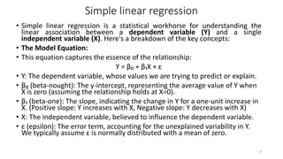
1) Regression analysis examines the relationship between a dependent variable and one or more independent variables. It was first developed by Francis Galton to study inheritance of traits. 2) Galton observed that the heights of children tended to "regress" toward the average height in the population, rather than matching their parents' exact heights. This was called "regression to mediocrity". 3) Simple linear regression analyzes the relationship between a single dependent variable and a single independent variable. It estimates the average value of the dependent variable based on the independent variable.

1. Bule Hora University
College of Business and Economics
Department of Economics
Chapter 2: Simple Linear Regression Model
By: Aschalew Shiferaw
1

2. Historical origin of the term “Regression”
• The term REGRESSION was introduced by Francis Galton
• Tendency for tall parents to have tall children and for short parents to have short
children, but the average height of children born from parents of a given height
tended to move (or regress) toward the average height in the population as a
whole. (F. Galton, “Family Likeness in Stature”)
2

3. Historical origin of the term “Regression”
• Galton’s Law was confirmed by Karl Pearson:
• The average height of sons of a group of tall fathers < their fathers’ height. And
the average height of sons of a group of short fathers > their fathers’ height.
Thus “regressing” tall and short sons alike toward the average height of all men.
(K. Pearson and A. Lee, “On the law of Inheritance”)
• By the words of Galton, this was “Regression to mediocrity”
3

4. Modern Interpretation of Regression Analysis
• Regression Analysis is concerned with the study of the dependence of one
variable (The Dependent Variable), on one or more other variable(s) (The
Explanatory Variable), with a view to estimating and/or predicting the
(population) mean or average value of the former in term of the known or
fixed (in repeated sampling) values of the latter.
4

5. Dependent Variable Y; Explanatory Variable Xs
1. Y = Son’s Height; X = Father’s Height
2. Y = Height of boys; X = Age of boys
3. Y = Personal Consumption Expenditure
X = Personal Disposable Income
4. Y = Demand; X = Price
5. Y = Rate of Change of Wages
X = Unemployment Rate
6. Y = Money/Income; X = Inflation Rate
7. Y = % Change in Demand; X = % Change in the advertising budget
8. Y = Crop yield; Xs = temperature, rainfall, sunshine, fertilizer
5

6. 1-4. Regression vs. Causation:
• Regression does not necessarily imply causation. A statistical
relationship cannot logically imply causation. “A statistical
relationship, however strong and however suggestive, can never
establish causal connection: our ideas of causation must come from
outside statistics, ultimately from some theory or other” (M.G.
Kendal and A. Stuart, “The Advanced Theory of Statistics”)
6

7. 1-5. Regression vs. Correlation
• Correlation Analysis: the primary objective is to measure the strength or
degree of linear association between two variables (both are assumed to
be random)
• Regression Analysis: we try to estimate or predict the average value of one
variable (dependent, and assumed to be stochastic) on the basis of the
fixed values of other variables (independent, and non-stochastic)
7

8. 1-6. Terminology and Notation
Dependent Variable

Explained Variable

Predictand

Regressand

Response

Endogenous
Explanatory Variable(s)

Independent Variable(s)

Predictor(s)

Regressor(s)

Stimulus or control variable(s)

Exogenous(es)
8

9. Simple linear regression
• Simple linear regression is a statistical workhorse for understanding the
linear association between a dependent variable (Y) and a single
independent variable (X). Here's a breakdown of the key concepts:
• The Model Equation:
• This equation captures the essence of the relationship:
Y = β₀ + β₁X + ε
• Y: The dependent variable, whose values we are trying to predict or explain.
• β₀ (beta-nought): The y-intercept, representing the average value of Y when
X is zero (assuming the relationship holds at X=0).
• β₁ (beta-one): The slope, indicating the change in Y for a one-unit increase in
X. (Positive slope: Y increases with X, Negative slope: Y decreases with X)
• X: The independent variable, believed to influence the dependent variable.
• ε (epsilon): The error term, accounting for the unexplained variability in Y.
We typically assume ε is normally distributed with a mean of zero.
9

10. Why do we need to include the stochastic (random) component, for
example in the consumption function?
1.Omission of variables: leads to misspecification problem. For
example, income is not the only determinants of consumption.
2.Vagueness of theory: The theory, if any, determining the behavior of Y may be,
and often is, incomplete. We might know for certain that weekly income X
influences weekly consumption expenditure Y, but we might be ignorant or
unsure about the other variables affecting Y. Therefore, ui may be used as a
substitute for all the excluded or omitted variables from the model
3.There may be measurement error in collecting data. We may use poor proxy
variables, inaccuracy in collection and measurement of sample data.
4. The functional form may not be correct. 10

11. Cont…
5. Erratic (random = unpredictable) human behaviour. Even if we succeed in
introducing all the relevant variables into the model, there is bound to be
some “intrinsic” randomness in individual Y’s that cannot be explained no
matter how hard we try. The disturbances, the u’s, may very well reflect this
intrinsic randomness.
6. Error of aggregation:- the sum of the parts may be different from the
whole.
11

12. Cont…
7.Sampling error: Consider a model relating Consumption (Y) with income
(X) of HHs. The sample we randomly choose to examine the R/ship may
turn out to be predominantly poor HHs. In such cases, our estimation of α
and β from this sample may not be as good as that from a balanced sample
group.
8.Unavailability of data: Even if we know what some of the excluded
variables are and therefore consider a multiple regression rather than a
simple regression, we may not have quantitative information about these
variables.
12

13. Cont….
• Thus, a full specification of a regression model should include a
specification of the probability distribution of the disturbance (error) term.
This information is given by what we call basic assumptions of the Classic
Linear Regression Model (CLRM).
• Consider the model
Here the subscript i refers to the ith observation. In CLRM, Yi and Xi are
observable while εi is not.
• If i refers to some point or period of time, then we speak of time series
data.
• On the other hand, if i refers to the ith individual, object, geographical
region, etc., then we speak of cross-sectional data.
i
Y = , i = 1,2,...,n
i i
X
  
 
13

14. Assumption of the classical linear regression
model
• The linear regression model is based on certain assumptions, some of
which refer to the distribution of the random variable ε, some to the
relationship b/n u and explanatory variables, and finally some refers
to the relationship b/n the explanatory variables themselves. We
will group the assumptions in two categories, (a) Stochastic
assumptions, (b) other assumptions.
• Stochastic Assumption of OLS
• Assumption 1: the true model is
• This Assumption states that the r/ship b/n Yi and Xi is linear, and that
the deterministic component( ) and the stochastic component
( ) are additive.
14
i i i
Y X
  
  
i
X
 

i


15. Cont…
Assumption 2: The mean of u in any particular period is Zero.𝜀 𝑢𝑖 =
0
This means that for each value of X, ε may assume various values,
some greater than zero and some smaller than zero, but if we consider
all the possible values of ε, for any given value of X, they would have an
average value equal to zero.
Assumption 3: The variance of is constant in each period
(Homoscedasticity)
The variance of about its mean is constant at all values of X. in
other words for all values of X, the ε ’s will show the same dispersion
around their mean.
Assumption 4: The variables has a normal distribution with mean
zero and variance 𝜎2
for all i (often written as: 𝜀𝑖~𝑁(0, 𝜎2
)
15
i

i

i


16. Cont…
• Assumption 5: the random term of different observations 𝑼𝒊, & 𝑼𝒋
are independent ( No error autocorrelation)
• This means that all the covariance of any 𝑼𝒊 with any other 𝑼𝒋 are equal to zero. The
value which the random term assumed in one period does not depend on the value which it
assumed in any other period.
Assumption 6: U is independent of explanatory variable
• The disturbance term is not correlated with the explanatory variable(s).
The u’s and the X’s do not tend to vary together; their covariance is zero.
𝑐𝑜𝑣 𝑿𝒊𝑼𝒋 = 0
16

17. Cont…
• Assumption 7: The explanatory variable(s) are measured without
error.
• u absorbs the influence of omitted variables and possibly error of
measurement in the y’s. that is, we will assume that the regressions
are error–free, while the values may or may not include errors of
measurements
  
 
 
 
cov( ) ( ) ( ) 0
( ) ( ) 0
( ) ( ) ( )
( )
( ) '
0
i i i i
i i i i
i i i i
i i
i i i
Xu E X E X u E u
E X E X u given E u
E X u E X E u
E X u
X E u giventhat the X s are fixed
   
  
 



17

18. Cont…
•Other assumptions
Assumption 8: the explanatory variables are not perfectly linearly correlated.
• If there is more than one explanatory variable in the r/ship it is assumed
that they are not perfectly correlated with each other. Indeed the
repressors should not even be strongly correlated, they should not be
highly multicollinear.
Assumption 9: the macro variables should be correctly aggregated.
• Usually the variables X and Y are aggregative variables, representing the
sum of individual items. For example, in consumption function C=bo+biY+u,
C is the sum of the expenditures of all consumers and Y is the sum of all
individual incomes.it is assumed that the appropriate aggregation
procedure has been adopted in compiling the aggregate variables.
18

19. cont
• Assumption 10: the r/ship being estimated is identified.
• It is assumed that the r/ship whose coefficients we want to estimate
has a unique mathematical form, that is it does not contain the same
variables as any other equation related to the one being investigated.
Assumption 11: the r/ship is correctly specified( no specification bias or
error).
Assumptions 12: The number of observations n must be greater than
the number of parameters to be estimated.
19

20. 20

21. Cont’d
21

22. 22

23. Methods of estimation
• Specifying the model and stating its underlying assumptions are the
first stage of any econometric application. The next step is the
estimation of the numerical values of the parameters of economic
relationships. The parameters of the simple linear regression model
can be estimated by various methods. Three of the most commonly
used methods are:
• Ordinary least square method (OLS)
• Maximum likelihood method (MLM)
• Method of moments (MM)
• But, here we will deal with the OLS and the MLM methods of
estimation.
23

24. The ordinary least square (OLS) method
• The model 𝑌𝑖 = 𝛼 + 𝛽𝑋𝑖 + 𝑈𝑖 is called the true relationship between
Y and X because Y and X represent their respective population value,
and are called the true parameters since they are estimated from the
population value of Y and X. But it is difficult to obtain the population
value of Y and X because of technical or economic reasons.
24

25. Cont’d
• So we are forced to take the sample value of Y and X. The parameters
estimated from the sample value of Y and X are called the estimators of the
true parameters 𝛼 and 𝛽 are symbolized as 𝛼 & 𝛽.
• The model 𝑌𝑖 = 𝛼 + 𝛽𝑋𝑖 + 𝑒𝑖, is called estimated relationship between Y
and X since 𝛼 & 𝛽 are estimated from the sample of Y and X and
represents the sample counterpart of the population random disturbance
𝑈𝑖.
25

26. Cont’d
26

27. 27

28. 28

29. 29

30. PROPERTIES OF OLS ESTIMATORS
• The ideal or optimum properties that the OLS estimates possess may be
summarized by well known theorem known as the Gauss-Markov Theorem.
• Statement of the theorem: “Given the assumptions of the classical linear
regression model, the OLS estimators, in the class of linear and unbiased
estimators, have the minimum variance, i.e. the OLS estimators are BLUE.
30

31. Cont’d
• An estimator is called BLUE if:
• Linear: a linear function of the random variable, such as, the dependent
variable Y.
• Unbiased: its average or expected value is equal to the true population
parameter.
• Minimum variance: It has a minimum variance in the class of linear and
unbiased estimators. An unbiased estimator with the least variance is known
as an efficient estimator.
• According to the Gauss-Markov theorem, the OLS estimators possess all the BLUE
properties. The detailed proof of these properties are presented below
31

32. Let’s proof these properties one by one.
32

33. b. Unbiasedness:
• Proposition: 𝛼 & 𝛽 are the unbiased estimators of the true parameters 𝜶 & 𝜷
• From your statistics course, you may recall that if 𝜃 is an estimator of 𝜃 then ∈
(𝜃) − 𝜃 = the amount of bias and if 𝜃 is the unbiased estimator 𝜃 of then bias ∈
(𝜃) − 𝜃 = 0 i.e. ∈ (𝜃) = 𝜃
• In our case, 𝛼 & 𝛽 are estimators of the true parameters 𝜶 & 𝜷. To show that
they are the unbiased estimators of their respective parameters means to prove
that: ∈ (𝛽) = 𝜷 , and ∈ 𝛼 = 𝛼.
33

34. Cont’d
34

35. Cont’d
35

36. 36

37. C. Minimum Variance
• OLS estimators possess a minimum variance, in the class of linear and
unbiased estimators. Proof it by yourself!
37

38. The variance of the random variable (Ui)
• You may observe that the variances of the OLS estimates involve 𝜎2,
which is the population variance of the random disturbance term. But
it is difficult to obtain the population data of the disturbance term
because of technical and economic reasons.
• Hence it is difficult to compute 𝜎2; this implies that variances of OLS
estimates are also difficult to compute. But we can compute these
variances if we take the unbiased estimate of 𝜎2
which is 𝜎2
computed from the sample value of the disturbance term ei from the
expression:
𝜎2 =
𝑒2
𝑛 − 2
38

39. 39

40. TESTS OF THE ‘GOODNESS OF FIT’ WITH R2
40
 R2
shows the percentage of total variation of the dependent variable that
can be explained by the changes in the explanatory variable(s) included in
the model.
 To elaborate this let’s draw a horizontal line corresponding to the mean
value of the dependent variable .
Y (see figure ‘d’ below).
 By fitting the line X
Y 1
0
ˆ
ˆ
ˆ 
 
 we try to obtain the explanation of the
variation of the dependent variable Y produced by the changes of the
explanatory variable X.

41. Cont’d
41
In summary:
Y
Y
e i
i
ˆ

 = deviation of the observation Yi from the regression line.
Y
Y
yi 
 = deviation of Y from its mean.
Y
Y
y 
 ˆ
ˆ = deviation of the regressed (predicted) value (Yˆ ) from the mean.

42. Cont’d
42

43. 43

44. Cont’d
44
From (2.48), RSS=TSS-ESS. Hence R2
becomes;
TSS
RSS
TSS
RSS
TSS
R 


 1
2
2
2
1
y
ei



 ………………………….…………(2.55)
From equation (2.55) we can drive;
)
56
.
2
(
)
1
( 2
2
2
































 R
y
e
RSS i
i
The limit of R2:
The value of R2
falls between zero and one. i.e. 1
0 2

 R

45. Cont’d
• Interpretation of R2
• Suppose , this means that the regression line gives a good fit to the
observed data since this line explains 90% of the total variation of the
Y value around their mean. The remaining 10% of the total variation
in Y is unaccounted for by the regression line and is attributed to the
factors included in the disturbance variable
45

46. 46
Hypothesis Testing on the Slope
and Intercept
• Three assumptions needed to apply procedures such as hypothesis
testing and confidence intervals. Model errors, i,
• are normally distributed
• are independently distributed
• have constant variance
i.e. i ~ NID(0, 2)

47. Cont’d
47

48. A. Standard error test
48

49. Cont….
49

50. Cont….
50

51. B. Student’s t-test
51

52. Cont….
52

53. Cont….
53

54. 54

55. Confidence interval
• To define how close the estimate to the true parameter, we must construct
confidence interval for the true parameter, in other words we must establish
limiting values around the estimate with in which the true parameter is expected
to lie within a certain “degree of confidence”.
• In this respect we say that with a given probability the population parameter will
be within the defined confidence interval (confidence limits).
55

56. Cont’d
• We choose a probability in advance and refer to it as confidence level
(interval coefficient). It is customarily in econometrics to choose the 95%
confidence level.
• This means that in repeated sampling the confidence limits, computed
from the sample, would include the true population parameter in 95% of
the cases. In the other 5% of the cases the population parameter will fall
outside the confidence interval.
56

57. How to Carry out a Hypothesis Test Using Confidence Intervals
1. Calculate , and , as before.
2. Choose a significance level, , (again the convention is 5%). This is equivalent to choosing a (1-)100%
confidence interval, i.e. 5% significance level = 95% confidence interval
3. Use the t-tables to find the appropriate critical value, which will again have n-2 degrees of freedom.
4. The confidence interval is given by
5. Perform the test: If the hypothesised value of  (*) lies outside the confidence interval, then reject the null
hypothesis that  = *, otherwise do not reject the null.
$
 $
 SE( $)
 SE( $)

))
ˆ
(
ˆ
),
ˆ
(
ˆ
( 


 SE
t
SE
t crit
crit 



57

58. Confidence Intervals Versus Tests of Significance
• Note that the Test of Significance and Confidence Interval approaches
always give the same answer.
• Under the test of significance approach, we would not reject H0 that  = * if the test
statistic lies within the non-rejection region, i.e. if
• Rearranging, we would not reject if
• But this is just the rule under the confidence interval approach.
 

 
t
SE
t
crit crit
$ *
( $)
 

)
ˆ
(
*
ˆ
)
ˆ
( 


 SE
t
SE
t crit
crit 






)
ˆ
(
ˆ
*
)
ˆ
(
ˆ 



 SE
t
SE
t crit
crit 





58

59. 59

60. 60

61. End of chapter 2
Thank You!!
61