chapter 2: Two-Variable Regression Analysis: Some Basic Ideas

1. Chapter 2
Two-Variable
Regression Analysis:
Some Basic Ideas

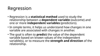
2. Regression
• Regression is a statistical method used to study the
relationship between a dependent variable (outcome) and
one or more independent variables (predictors).
• In simple terms, it helps us understand how changes in one
variable are associated with changes in another.
• The goal is often to predict the value of the dependent
variable based on known values of the independent
variable(s), or to measure the strength and direction of the
relationship.

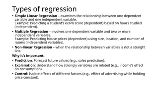
3. Types of regression
• Simple Linear Regression – examines the relationship between one dependent
variable and one independent variable.
Example: Predicting a student’s exam score (dependent) based on hours studied
(independent).
• Multiple Regression – involves one dependent variable and two or more
independent variables.
Example: Predicting house prices (dependent) using size, location, and number of
rooms (independent variables).
• Non-linear Regression – when the relationship between variables is not a straight
line.
Why it’s important:
• Prediction: Forecast future values (e.g., sales prediction).
• Explanation: Understand how strongly variables are related (e.g., income’s effect
on consumption).
• Control: Isolate effects of different factors (e.g., effect of advertising while holding
price constant).

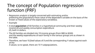
4. The concept of Population regression
function (PRF)
• Regression analysis is largely concerned with estimating and/or
predicting the (population) mean value of the dependent variable on the basis of the
known or fixed values of the explanatory variable(s).
• Example
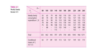
• A total population of 60 families in a hypothetical community and their weekly
income (X) and weekly consumption expenditure
(Y), both in dollars.
• The 60 families are divided into 10 income groups (from $80 to $260)
and the weekly expenditures of each family in the various groups are as shown in
the table.
• Therefore, we have 10 fixed values of X and the corresponding Y values against each
of the
X values; so to speak, there are 10 Y subpopulations.

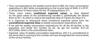
6. • Thus, corresponding to the weekly income level of $80, the mean consumption
expenditure is $65, while corresponding to the income level of $200, it is $137.
In all we have 10 mean values for the 10 subpopulations of Y.
• These mean values conditional expected values, as they depend
on the given values of the (conditioning) variable X. Symbolically, we denote
them as E(Y | X), which is read as the expected value of Y given the value of X.
• It is important to distinguish these conditional expected values from the
unconditional expected value of weekly consumption expenditure, E(Y).
• If we add the weekly consumption expenditures for all the 60 families in the
population and divide this number by 60, we get the number $121.20
($7272/60), which is the unconditional mean.
• Expected, value of weekly consumption expenditure, E(Y); it is unconditional in
the sense that in arriving at this number we have disregarded the income levels
of the various families.

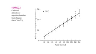
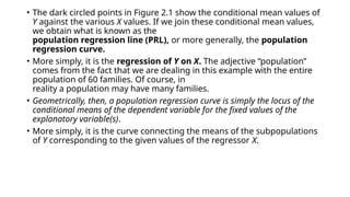
8. • The dark circled points in Figure 2.1 show the conditional mean values of
Y against the various X values. If we join these conditional mean values,
we obtain what is known as the
population regression line (PRL), or more generally, the population
regression curve.
• More simply, it is the regression of Y on X. The adjective “population”
comes from the fact that we are dealing in this example with the entire
population of 60 families. Of course, in
reality a population may have many families.
• Geometrically, then, a population regression curve is simply the locus of the
conditional means of the dependent variable for the fixed values of the
explanatory variable(s).
• More simply, it is the curve connecting the means of the subpopulations
of Y corresponding to the given values of the regressor X.

9. PRF
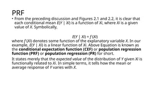
• From the preceding discussion and Figures 2.1 and 2.2, it is clear that
each conditional mean E(Y | Xi) is a function of Xi, where Xi is a given
value of X. Symbolically,
E(Y | Xi) = f (Xi)
where f (Xi) denotes some function of the explanatory variable X. In our
example, E(Y | Xi) is a linear function of Xi. Above Equation is known as
the conditional expectation function (CEF) or population regression
function (PRF) or population regression (PR) for short.
It states merely that the expected value of the distribution of Y given Xi is
functionally related to Xi. In simple terms, it tells how the mean or
average response of Y varies with X.

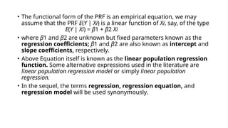
10. • The functional form of the PRF is an empirical equation, we may
assume that the PRF E(Y | Xi) is a linear function of Xi, say, of the type
E(Y | Xi) = β1 + β2 Xi
• where β1 and β2 are unknown but fixed parameters known as the
regression coefficients; β1 and β2 are also known as intercept and
slope coefficients, respectively.
• Above Equation itself is known as the linear population regression
function. Some alternative expressions used in the literature are
linear population regression model or simply linear population
regression.
• In the sequel, the terms regression, regression equation, and
regression model will be used synonymously.

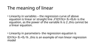
11. The meaning of linear
• Linearity in variables – the regression curve of above
equation is linear or straight line .if E(Y/Xi)= ß1+ß2Xi2
is the
equation, as the power of the variable Xi is 2 ,this cannot be
a linear equation.
• Linearity in parameters- the regression equation is
E(Y/Xi)= ß1+ß2 2
Xi ,this is an example of non linear regression
model

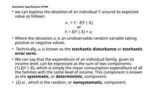
12. Stochastic Specification of PRF
• we can express the deviation of an individual Yi around its expected
value as follows:
u i = Yi - E(Y | Xi)
or
Yi = E(Y | Xi) + ui
• Where the deviation ui is an unobservable random variable taking
positive or negative values.
• Technically, ui is known as the stochastic disturbance or stochastic
error term.
• We can say that the expenditure of an individual family, given its
income level, can be expressed as the sum of two components:
(1) E(Y | Xi), which is simply the mean consumption expenditure of all
the families with the same level of income. This component is known
as the systematic, or deterministic, component.
• (2) ui , which is the random, or nonsystematic, component.

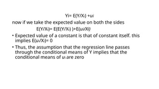
13. Yi= E(Y/Xi) +ui
now if we take the expected value on both the sides
E(Y/Xi)= E(E(Y/Xi) )+E(ui/Xi)
• Expected value of a constant is that of constant itself. this
implies E(ui/Xi)= 0
• Thus, the assumption that the regression line passes
through the conditional means of Y implies that the
conditional means of ui are zero

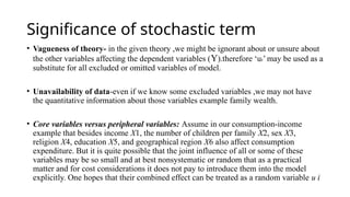
14. Significance of stochastic term
• Vagueness of theory- in the given theory ,we might be ignorant about or unsure about
the other variables affecting the dependent variables (Y).therefore ‘ui’ may be used as a
substitute for all excluded or omitted variables of model.
• Unavailability of data-even if we know some excluded variables ,we may not have
the quantitative information about those variables example family wealth.
• Core variables versus peripheral variables: Assume in our consumption-income
example that besides income X1, the number of children per family X2, sex X3,
religion X4, education X5, and geographical region X6 also affect consumption
expenditure. But it is quite possible that the joint influence of all or some of these
variables may be so small and at best nonsystematic or random that as a practical
matter and for cost considerations it does not pay to introduce them into the model
explicitly. One hopes that their combined effect can be treated as a random variable u i

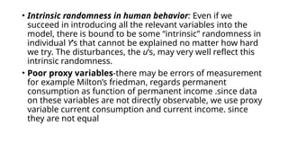
15. • Intrinsic randomness in human behavior: Even if we
succeed in introducing all the relevant variables into the
model, there is bound to be some “intrinsic” randomness in
individual Y’s that cannot be explained no matter how hard
we try. The disturbances, the u’s, may very well reflect this
intrinsic randomness.
• Poor proxy variables-there may be errors of measurement
for example Milton’s friedman, regards permanent
consumption as function of permanent income .since data
on these variables are not directly observable, we use proxy
variable current consumption and current income. since
they are not equal

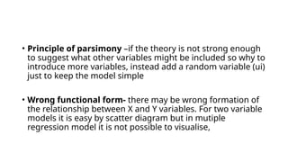
16. • Principle of parsimony –if the theory is not strong enough
to suggest what other variables might be included so why to
introduce more variables, instead add a random variable (ui)
just to keep the model simple
• Wrong functional form- there may be wrong formation of
the relationship between X and Y variables. For two variable
models it is easy by scatter diagram but in mutiple
regression model it is not possible to visualise,

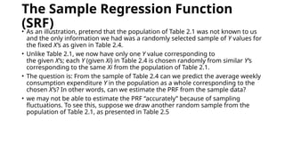
17. The Sample Regression Function
(SRF)
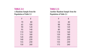
• As an illustration, pretend that the population of Table 2.1 was not known to us
and the only information we had was a randomly selected sample of Y values for
the fixed X’s as given in Table 2.4.
• Unlike Table 2.1, we now have only one Y value corresponding to
the given X’s; each Y (given Xi) in Table 2.4 is chosen randomly from similar Y’s
corresponding to the same Xi from the population of Table 2.1.
• The question is: From the sample of Table 2.4 can we predict the average weekly
consumption expenditure Y in the population as a whole corresponding to the
chosen X’s? In other words, can we estimate the PRF from the sample data?
• we may not be able to estimate the PRF “accurately” because of sampling
fluctuations. To see this, suppose we draw another random sample from the
population of Table 2.1, as presented in Table 2.5

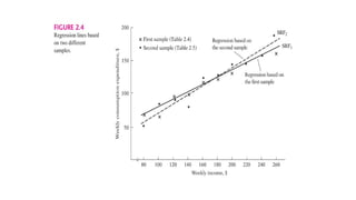
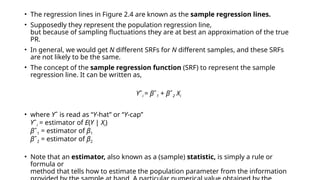
20. • The regression lines in Figure 2.4 are known as the sample regression lines.
• Supposedly they represent the population regression line,
but because of sampling fluctuations they are at best an approximation of the true
PR.
• In general, we would get N different SRFs for N different samples, and these SRFs
are not likely to be the same.
• The concept of the sample regression function (SRF) to represent the sample
regression line. It can be written as,
Yˆi = βˆ1 + βˆ2 Xi
• where Yˆ is read as “Y-hat’’ or “Y-cap’’
Yˆi = estimator of E(Y | Xi)
βˆ1 = estimator of β1
βˆ2 = estimator of β2
• Note that an estimator, also known as a (sample) statistic, is simply a rule or
formula or
method that tells how to estimate the population parameter from the information

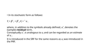
21. • In its stochastic form as follows:
Yi = βˆ1 + βˆ2 Xi + ˆ u i
where, in addition to the symbols already defined, uˆi denotes the
(sample) residual term.
Conceptually uˆi is analogous to ui and can be regarded as an estimate
of ui .
It is introduced in the SRF for the same reasons as ui was introduced in
the PRF.