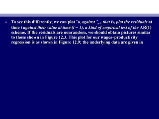
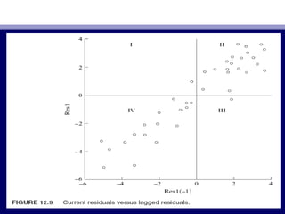
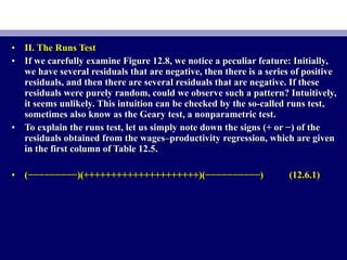
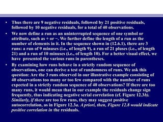
Downloaded 21 times

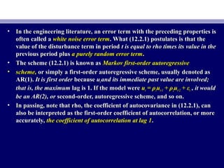
![• THE NATURE OF THE PROBLEMTHE NATURE OF THE PROBLEM
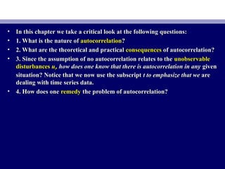
• Autocorrelation may be defined as “Autocorrelation may be defined as “correlation between members of series ofcorrelation between members of series of
observations ordered in timeobservations ordered in time [as in time series data] or[as in time series data] or spacespace [as in cross-[as in cross-
sectional data].’’ the CLRM assumes that:sectional data].’’ the CLRM assumes that:
• E(uE(uiiuujj ) = 0) = 0 i ≠ ji ≠ j (3.2.5)(3.2.5)
• Put simply, the classical model assumes that the disturbance term relatingPut simply, the classical model assumes that the disturbance term relating
to any observation is not influenced by the disturbance term relating to anyto any observation is not influenced by the disturbance term relating to any
other observation.other observation.
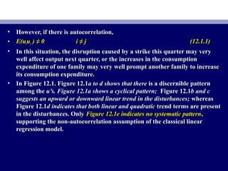
• For example, if we are dealing with quarterly time series data involving theFor example, if we are dealing with quarterly time series data involving the
regression ofregression of output on labor and capitaloutput on labor and capital inputs and if, say, there is a laborinputs and if, say, there is a labor
strike affecting output in one quarter, there is no reason to believe that thisstrike affecting output in one quarter, there is no reason to believe that this
disruption will be carried over to the next quarter. That is, if output is lowerdisruption will be carried over to the next quarter. That is, if output is lower
this quarter, there is no reason to expect it to be lower next quarter.this quarter, there is no reason to expect it to be lower next quarter.
Similarly, if we are dealing with cross-sectional data involving theSimilarly, if we are dealing with cross-sectional data involving the
regression ofregression of family consumptionfamily consumption expenditure on family income, the effect ofexpenditure on family income, the effect of
an increase of one family’s income on its consumption expenditure is notan increase of one family’s income on its consumption expenditure is not
expected to affect the consumption expenditure of another family.expected to affect the consumption expenditure of another family.](https://image.slidesharecdn.com/econometricsch13-160908053110/85/Econometrics-ch13-3-320.jpg)

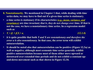
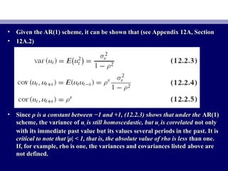
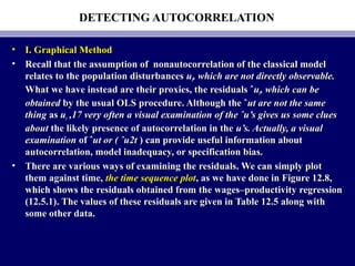
![• Now under the AR(1) scheme, it can be shown that the variance of thisNow under the AR(1) scheme, it can be shown that the variance of this
estimator is:estimator is:
• A comparison of (12.2.8) with (12.2.7) shows the former is equal to the latterA comparison of (12.2.8) with (12.2.7) shows the former is equal to the latter
times a term that depends ontimes a term that depends on ρ as well as the sample autocorrelationsρ as well as the sample autocorrelations
between the values taken by the regressorbetween the values taken by the regressor X at various lags. And in generalX at various lags. And in general
we cannot foretell whether var (we cannot foretell whether var (βˆ2) is less than or greater than var (βˆ2)AR1βˆ2) is less than or greater than var (βˆ2)AR1
[but see Eq. (12.4.1) below]. Of course, if rho is zero, the two formulas will[but see Eq. (12.4.1) below]. Of course, if rho is zero, the two formulas will
coincide, as they should (why?). Also, if the correlations among thecoincide, as they should (why?). Also, if the correlations among the
successive values of the regressor are very small, the usual OLS variance ofsuccessive values of the regressor are very small, the usual OLS variance of
the slope estimator will not be seriously biased. But, as a general principle,the slope estimator will not be seriously biased. But, as a general principle,
the two variances will not be the same.the two variances will not be the same.](https://image.slidesharecdn.com/econometricsch13-160908053110/85/Econometrics-ch13-21-320.jpg)
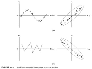
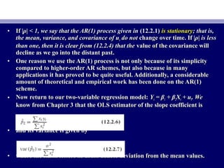
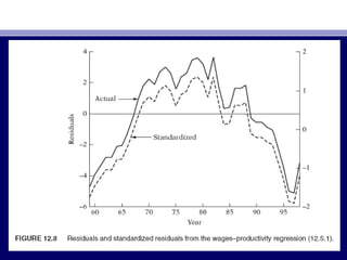
![• To give some idea about the difference between the variances given inTo give some idea about the difference between the variances given in
(12.2.7) and (12.2.8), assume that the regressor(12.2.7) and (12.2.8), assume that the regressor X also follows the first-orderX also follows the first-order
autoregressive scheme with a coefficient of autocorrelation ofautoregressive scheme with a coefficient of autocorrelation of r. Then it canr. Then it can
be shown that (12.2.8) reduces to:be shown that (12.2.8) reduces to:
• var (var (βˆ2)βˆ2)AR(1) =AR(1) = σ2σ2 x2 t 1 + rx2 t 1 + rρρ 1 −1 − rrρ =ρ = var (var (βˆ2)βˆ2)OLS 1 + rOLS 1 + rρρ 1 −1 − rrρ (12.2.9)ρ (12.2.9)
• If, for example,If, for example, r = 0.6 and ρ = 0.8, using (12.2.9) we can check thatr = 0.6 and ρ = 0.8, using (12.2.9) we can check that varvar
((βˆ2)AR1 = 2.8461 var (βˆ2)OLS. To put it another way, var (βˆ2)OLS = 1βˆ2)AR1 = 2.8461 var (βˆ2)OLS. To put it another way, var (βˆ2)OLS = 1
22.8461var (βˆ2)AR1 = 0.3513 var (βˆ2)AR1 . That is, the usual OLS formula.8461var (βˆ2)AR1 = 0.3513 var (βˆ2)AR1 . That is, the usual OLS formula
[i.e.,[i.e., (12.2.7)] will underestimate the variance of ((12.2.7)] will underestimate the variance of (βˆ2)AR1 by about 65βˆ2)AR1 by about 65
percent. Aspercent. As you will realize, this answer is specific for the given values ofyou will realize, this answer is specific for the given values of rr
and ρ. But theand ρ. But the point of this exercise is to warn you that a blind applicationpoint of this exercise is to warn you that a blind application
of the usual OLS formulas to compute the variances and standard errors ofof the usual OLS formulas to compute the variances and standard errors of
the OLS estimators could give seriously misleading results.the OLS estimators could give seriously misleading results.](https://image.slidesharecdn.com/econometricsch13-160908053110/85/Econometrics-ch13-22-320.jpg)
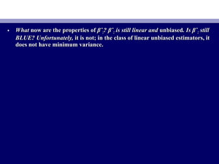
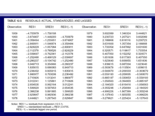
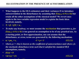
![• Now letNow let
• N = total number of observations = N1 + N2N = total number of observations = N1 + N2
• N1 = number of + symbols (i.e., + residuals)N1 = number of + symbols (i.e., + residuals)
• N2 = number of − symbols (i.e., − residuals)N2 = number of − symbols (i.e., − residuals)
• R = number of runsR = number of runs
• Note: N = N1 + N2.Note: N = N1 + N2.
• If the null hypothesis of randomness is sustainable, followingIf the null hypothesis of randomness is sustainable, following
the properties of the normal distribution, we should expect thatthe properties of the normal distribution, we should expect that
Prob [Prob [E(R) − 1.96σR ≤ R ≤ E(R) + 1.96σR] = 0.95E(R) − 1.96σR ≤ R ≤ E(R) + 1.96σR] = 0.95 (12.6.3)(12.6.3)](https://image.slidesharecdn.com/econometricsch13-160908053110/85/Econometrics-ch13-36-320.jpg)
![• Using the formulas given in (12.6.2), we obtainUsing the formulas given in (12.6.2), we obtain
• The 95% confidence interval forThe 95% confidence interval for R in our example is thus:R in our example is thus:
[10[10.975 ± 1.96(3.1134)] = (4.8728, 17.0722).975 ± 1.96(3.1134)] = (4.8728, 17.0722)](https://image.slidesharecdn.com/econometricsch13-160908053110/85/Econometrics-ch13-37-320.jpg)


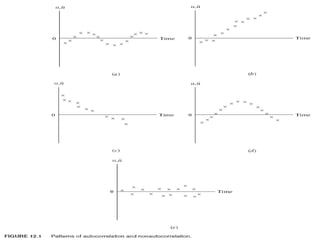
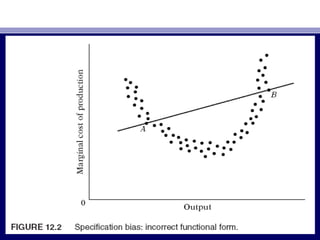
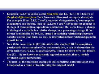
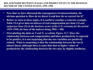
The document discusses the nature and causes of autocorrelation in regression models. Autocorrelation occurs when the error terms are correlated over time or between observations, violating the independence assumption of classical linear regression models. It can be caused by inertia in time series, omitted variables, incorrect functional forms, lags between dependent and independent variables, and data manipulation or transformation. Addressing autocorrelation is important as it can invalidate statistical tests and estimates in regression analysis.