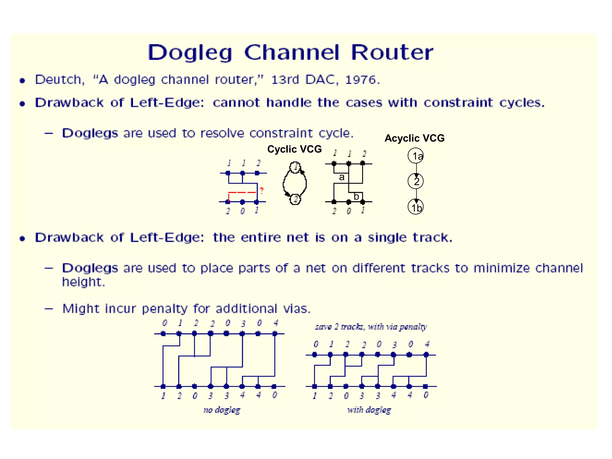
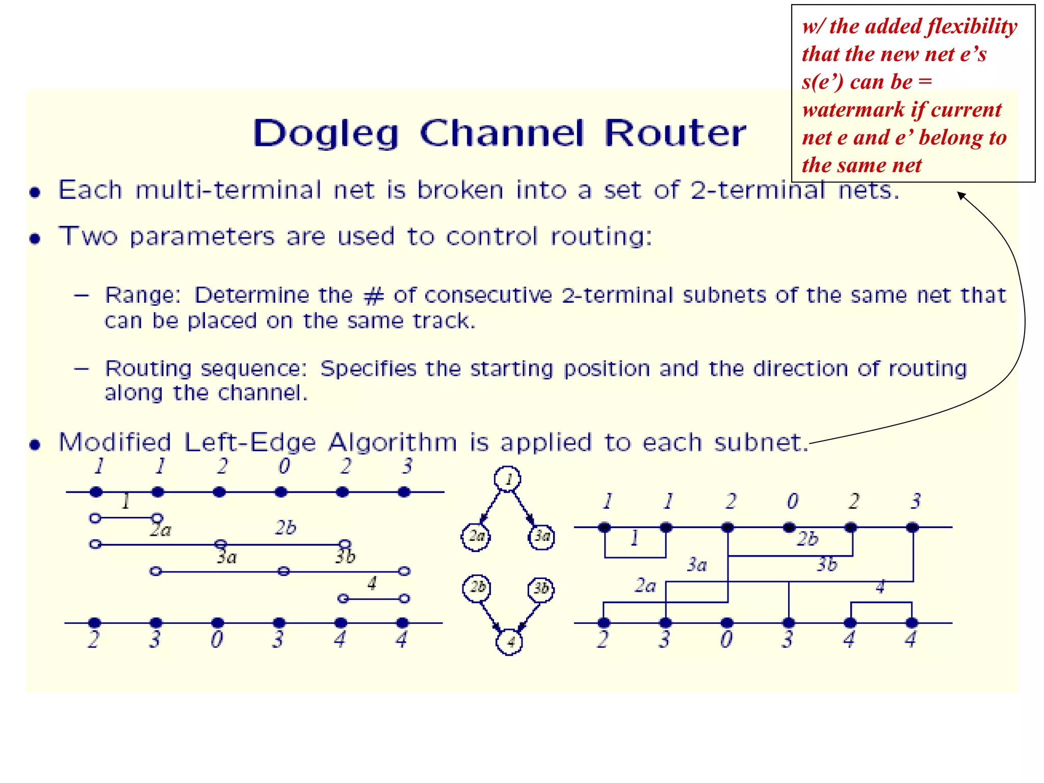
The document provides an overview of global and detailed routing in VLSI design. It discusses how global routing determines routing regions and channels while minimizing congestion and meeting timing constraints. Detailed routing then determines the exact routes and layers for each net within the given channels. Different routing algorithms are categorized, including graph search, hierarchical, and maze routing approaches. Concepts like grids, edge capacities, and Steiner trees are also summarized.

1. General Routing Overview
and Channel Routing
Shantanu Dutt
ECE Dept.
UIC

2. References and Copyright
(cont.)
• Slides used: (Modified by Shantanu Dutt when necessary)
– [©Sarrafzadeh] © Majid Sarrafzadeh, 2001;
Department of Computer Science, UCLA
– [©Sherwani] © Naveed A. Sherwani, 1992
(companion slides to [She99])
– [©Keutzer] © Kurt Keutzer, Dept. of EECS,
UC-Berekeley
http://www-cad.eecs.berkeley.edu/~niraj/ee244/index.htm
– [©Gupta] © Rajesh Gupta
UC-Irvine
http://www.ics.uci.edu/~rgupta/ics280.html
– [©Kang] © Steve Kang, UIUC http://www.ece.uiuc.edu/ece482/
– [©Bazargan] © Kia Bazargan

3. Routing
• Problem
– Given a placement, and a fixed number of metal layers, find a
valid pattern of horizontal and vertical wires that connect the
terminals of the nets
– Levels of abstraction:
• Global routing
• Detailed routing
• Objectives
– Cost components:
• Area (channel width) – min congestion in prev levels helped
• Wire delays – timing minimization in previous levels
• Number of layers (fewer layers  less expensive)
• Additional cost components: number of bends, vias
©Bazargan

4. Metal layer 1
Via
Routing Anatomy
Top
view
3D
view
Metal layer 2
Metal layer 3
Symbolic
Layout
Note: Colors used
in this slide are not
standard
©Bazargan

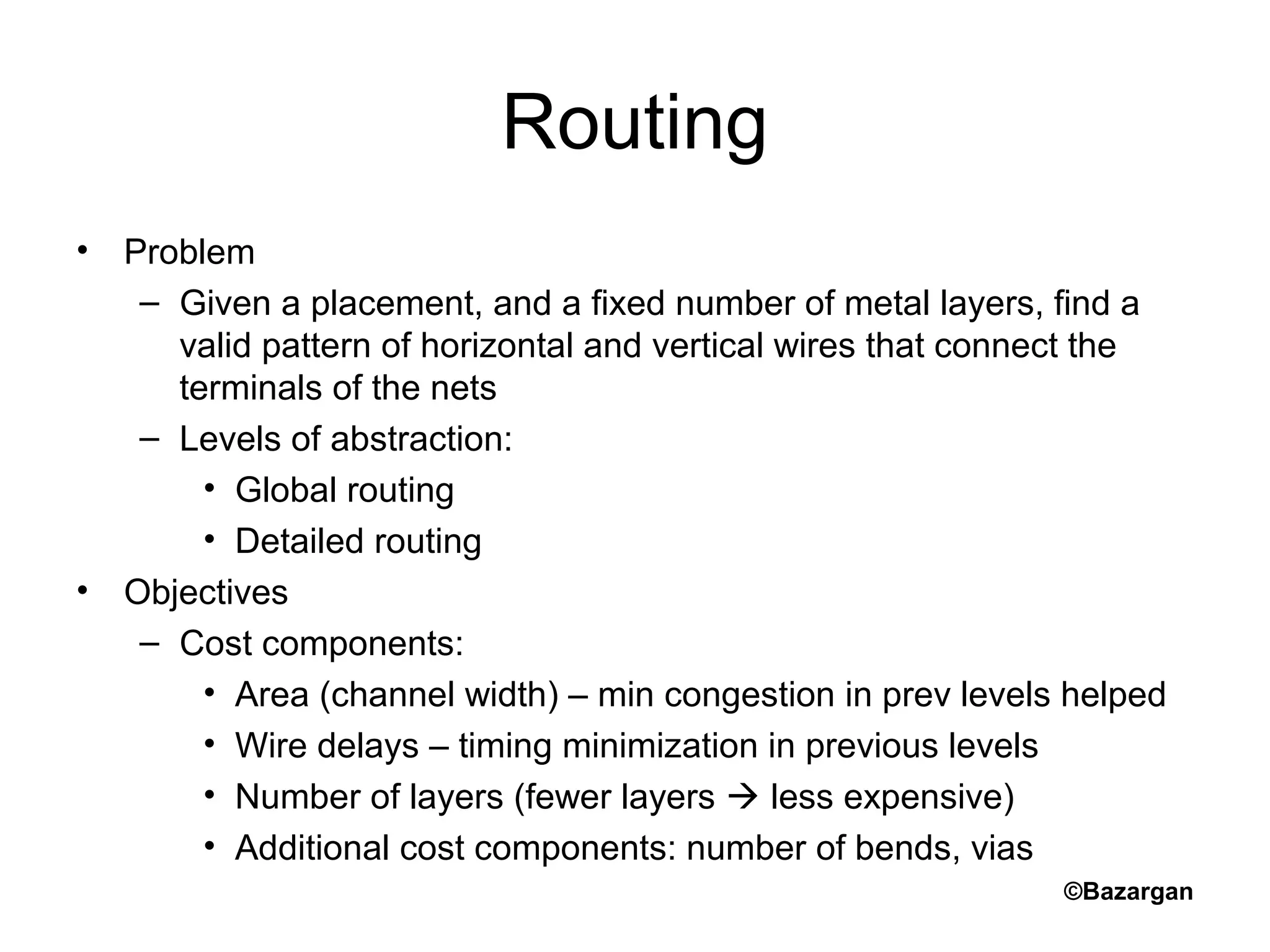
5. Global vs. Detailed Routing
• Global routing
– Input: detailed placement, with exact terminal
locations
– Determine “channel” (routing region) for each
net
– Objective: minimize area (congestion), and
timing (approximate)
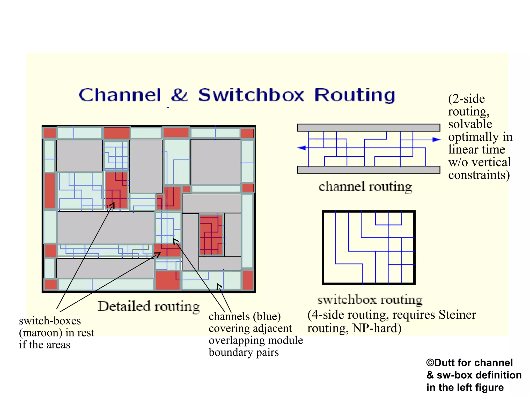
• Detailed routing
– Input: channels and approximate routing from
the global routing phase
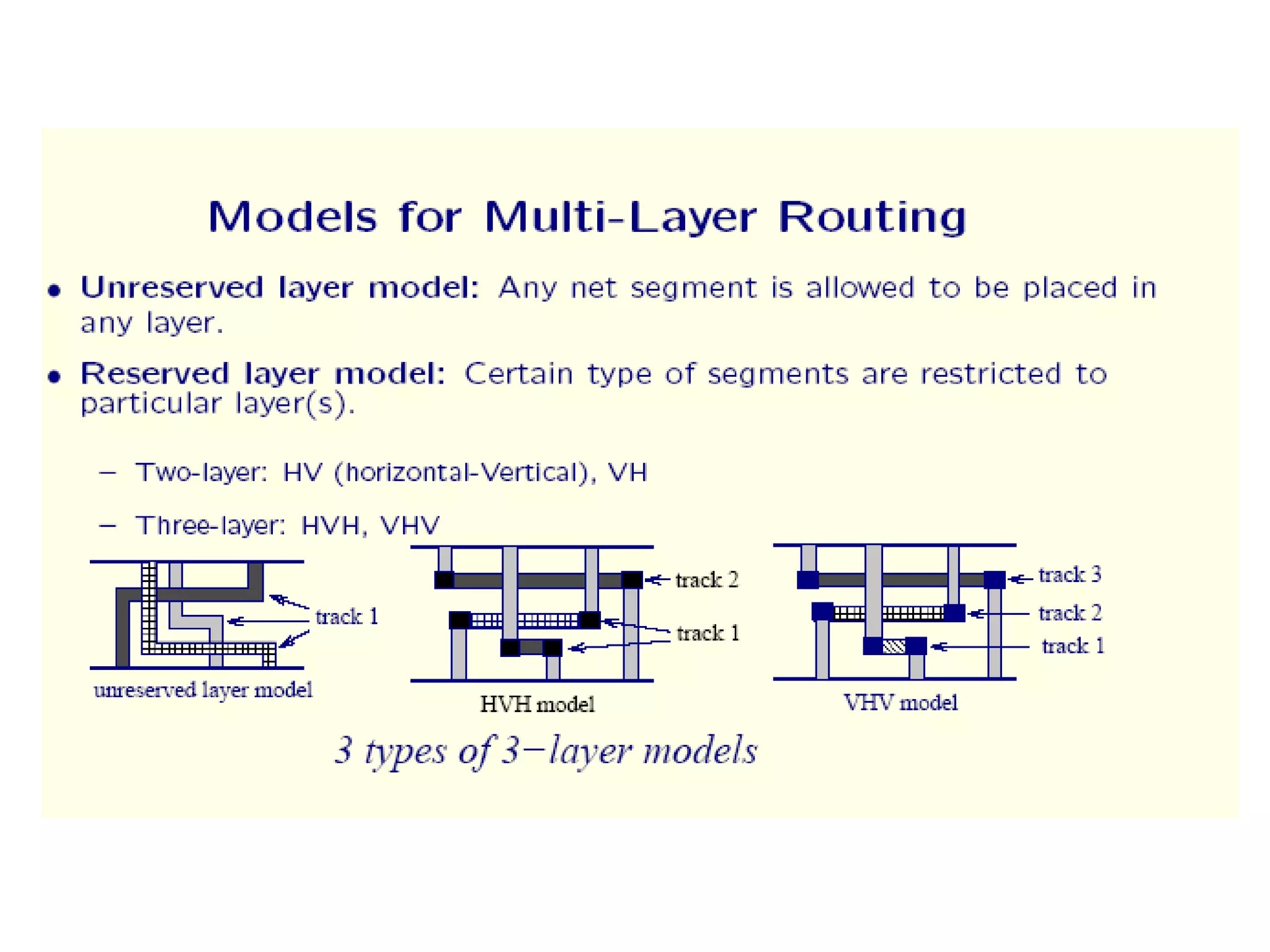
– Determine the exact route and layers for each
net
– Objective: valid routing, minimize area
(congestion), meet timing constraints
– Additional objectives: min via, power
Figs. [©Sherwani]

6. Taxonomy of VLSI Routers
[©Keutzer]
Graph Search
Steiner
Iterative
Hierarchical Greedy Left-Edge
River
Switchbox
Channel
Maze
Line Probe
Line Expansion
Restricted
General
Purpose
Clock
Specialized
Power/Gnd
Routers
DetailedGlobal
Maze

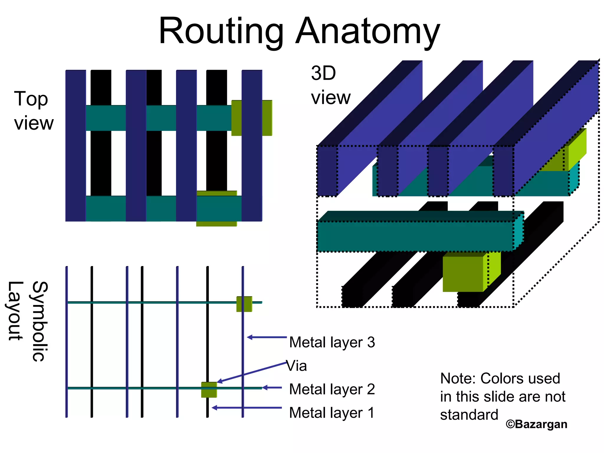
7. Global Routing
• Stages
– Routing region definition
– Routing region ordering
– Steiner-tree / area routing
• Grid
– Tiles super-imposed on placement
– Regular or irregular
– Smaller problem to solve,
higher level of abstraction
– Terminals at center of grid tiles
• Edge capacity
– Number of nets that can pass a certain
grid edge (aka congestion)
– On edge Eij,
Capacity(Eij) ≥ Congestion(Eij)
• Steiner routing is generally performed on the
routing graph using edge lengths as cost and
considering edge capacities
M1
M2
M3
[©Sarrafzadeh]

8. Grid Graph
• Course or fine-grain
• Vertices: routing regions, edges: route exists?
• Weights on edges
– How costly is to use that edge
– Could vary during the routing (e.g., for congestion)
– Horizontal / vertical might have different weights
[©Sherwani]
t1 t2 t3
t4
t1 t2 t3
t4
1 1 1
1 1 1
2 2 1 1
t1 t3
t4
t2

9. Global Routing – Graph Search
• Good for two-terminal nets
• Build grid graph (Coarse? Fine?)
• Use graph search algorithms, e.g., Dijkstra
• Iterative: route nets one by one
• How to handle:
– Congestion?
– Critical nets?
• Order of the nets to route?
– Net criticality
– Half-perimeter of the bounding box
– Number of terminals
©Bazargan

10. (4-side routing, requires Steiner
routing, NP-hard)
(2-side
routing,
solvable
optimally in
linear time
w/o vertical
constraints)
channels (blue)
covering adjacent
overlapping module
boundary pairs
switch-boxes
(maroon) in rest
if the areas
©Dutt for channel
& sw-box definition
in the left figure

15. • A cycle in the
VCG  an
unroutable
placement
unless a net
can be routed
on more than 1
track
• Otherwise,
depth of VCG is
lower bound on
channel density

19. Case 2a:
Closest non-ov
net to e crosses L
Case 2b:
Closest non-ov
net to e does not
cross L
L
e: Most recently
routed net
L’
e: Most recently
routed net
L
Optimality of the Left Edge Algorithm
Case 1: Max density line L cuts e Case 2: Max density line L does not cut e
• In Case 1, the density of L reduces by 1 after current track t (e is on t) is routed
• In Case 2, let e’ be the net not overlapping e & whose s(e’) is closest to e(e).
• Case 2a: If e’ crosses L, then since e’ will be on t, density of L reduces by 1 after t is routed
• Case 2b: If not, then the set S(L) of all other nets crossing L are overlapping w/ e (otherwise
one of them will be e’ and crossing L, and we will not be in Case 2b). Then there exists
another cut line L’ that cuts S(L) and e, and thus have density > density of L, and we reach a
contradiction (that L is the max density line)
• Thus after current track t is routed, the density of L reduces by 1. This applies to all max density
lines. Thus # of tracks needed = density of initial max density line which is a lower bound on #
tracks. Hence the Left-Edge algorithm is optimal in the # of tracks
e’
e’
s(e) e(e)
s(e’)
s(e’)
S(L)
©Dutt

20. Update the VCG by deleting all Ij ‘’s (and their arcs) routed in track t-1 > 0;
(no arcs in the
VCG incoming to Ij)

22. 1a
2
1b
b
a
Acyclic VCG
Cyclic VCG

23. w/ the added flexibility
that the new net e’s
s(e’) can be =
watermark if current
net e and e’ belong to
the same net