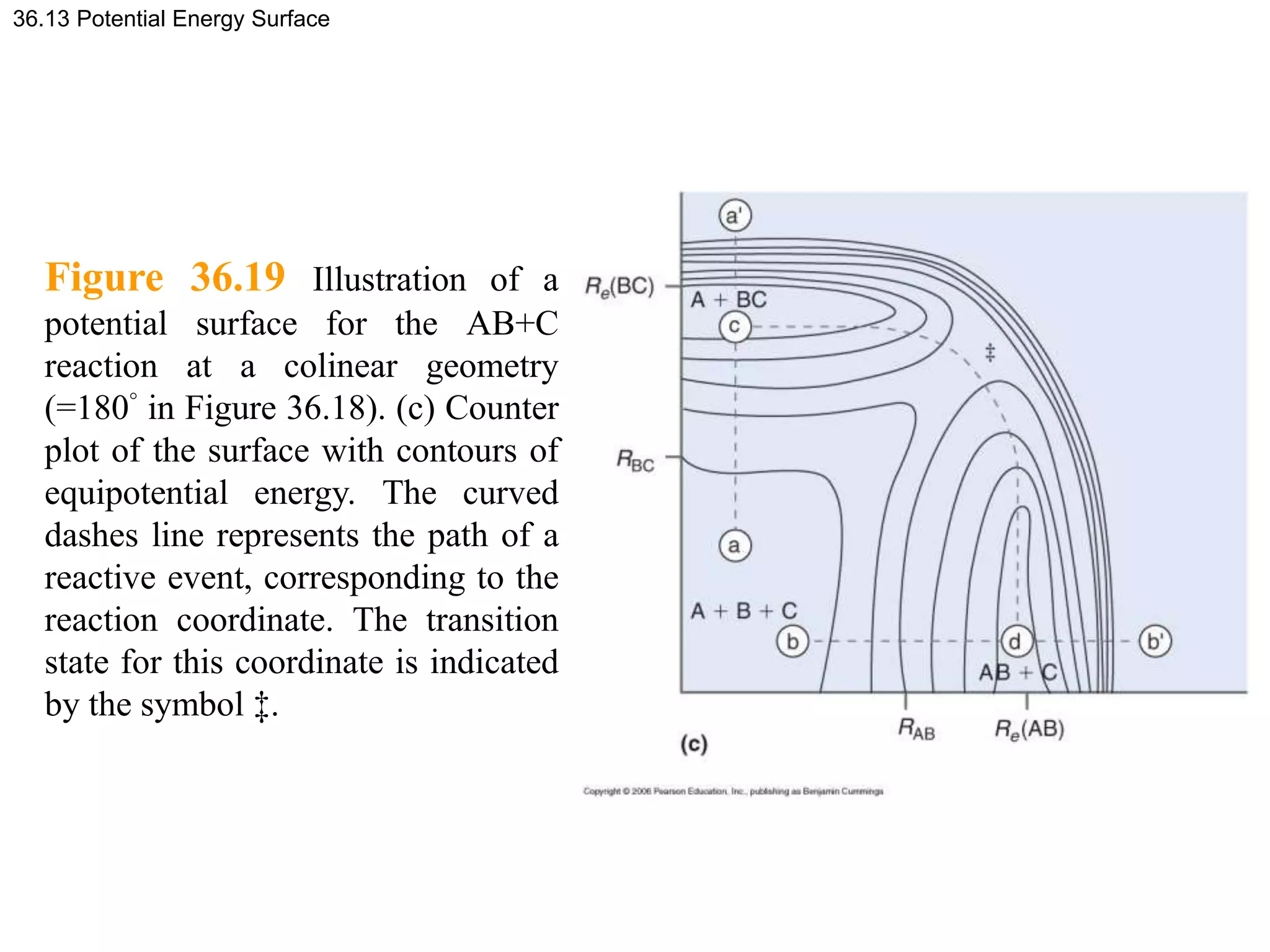
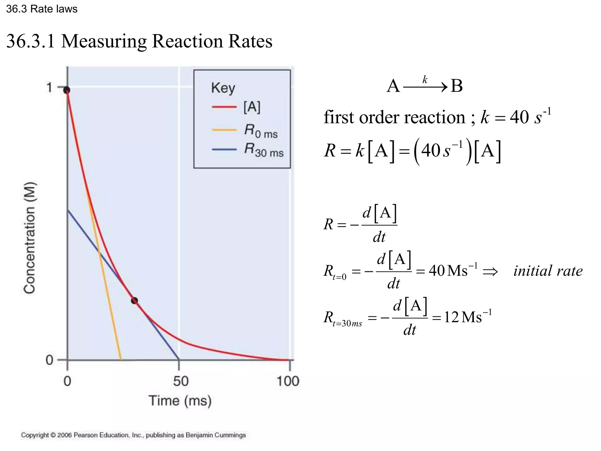
This document discusses elementary chemical kinetics and reaction rates. It defines reaction rate and rate laws. Reaction rate is the change in concentration of a reactant or product over time. The rate of a reaction is often proportional to the concentrations of reactants raised to a power defined by the reaction order. Reaction orders are determined experimentally and have no relation to stoichiometric coefficients. Integrated rate laws relate the concentrations of reactants and products over time for reactions of different orders (zero, first, second). Examples are provided to demonstrate determining reaction order from rate data and calculating time for specific conversions using integrated rate laws.

1. Chapter 36
Elementary Chemical
Kinetics
Engel & Reid

2. Figure 36.1
Figure 36.1 Concentration as a function of time for the conversion of
reactant A into product B. The concentration of A at time 0 is [A]0, and
the concentration of B is zero. As the reaction proceeds, the loss of A
results in the production of B.

3. 36.2 reaction rate
0
A B C+ D
The number of moles os a species during any point of the reaction
:advancement of the reaction
1
Reaction rate
Reaction rate in intensive expression R=
i i i
i
i
i
i
a b c d
n n v
dn d
v
dt dt
dn
d
Rate
dt v dt
 


  
 

 
rate 1 1 1 [ ]
V
i
i i
dn d i
V v dt v dt
 
 
 
 
2 5
2 2
2 (g) 2 (g) 2 5 (g)
N O
NO O
4NO O 2N O
1 1
4 2
dn
dn dn
Rate
dt dt dt
 
    
Example

4. 36.3 rate laws
Rate law : R = k [A]a
[B]b
...
Rate Constant
Reaction
order
• The rate of reaction is often found to be proportional to the molar
concentrations of the reactants raised to a simple power.
• It cannot be overemphasized that reaction orders have no relation
to stoichiometric coefficients, and they are determined by
experiment.

5. 36.3 Rate laws

6. 36.3 Rate laws
36.3.1 Measuring Reaction Rates
    
-1
1
A B
first order reaction ; 40
A 40 A
k
k s
R k s



 
 
 
 
1
0
1
30
A
A
40Ms
A
12Ms
t
t ms
d
R
dt
d
R initial rate
dt
d
R
dt




 
   
  

7. 36.3.2 Determining Reaction Orders
A + B C
[ ] [ ]
k
R k A B
a b



Strategy 1. Isolation method
The reaction is performed with all species but one in excess.
Under these conditions, only the concentration of one species will
vary to a significant extent during the reaction.
R = k’[B]b

8. 36.3.2 Determining Reaction Orders
Strategy 2. Method of initial rates
The concentration of a single reactant is changed while
holding all other concentrations constant, and the initial
rate of the reaction is determined.
A + B C
[ ] [ ]
k
R k A B
a b



 
 
1 0
1 1
2 2 0 2
1 1
2 2
A
[A] [B]
[A] [B] [A]
A
ln ln
[A]
k
R
R k
R
R
a
a b
a b
a
 
   
 
 
 
 
  
   
   

9. Example Problem 36.2
Using the following data for the reaction illustrated in equation
36.13. Determine the order of the reaction with respect to A and
B, and the rate constant for the reaction
[A] (M) [B] (M) Initial Rate (Ms-1)
2.3010-4 3.1010-5 5.2510-4
4.6010-4 6.2010-5 4.2010-3
9.2010-4 6.2010-5 1.7010-2

10.  
3 4
2 4
2
1 1 1
2
2 2 2
2
4 4 5
3 4 5
2
2
4 -1 4
4.20 10 4.60 10
ln ln 2
1.70 10 9.20 10
[A] [B]
[A] [B]
5.25 10 2.30 10 3.10 10
1
4.20 10 4.60 10 6.20 10
[A] [B]
5.2 10 Ms 2.3 10 M 3.1
R k
R k
R k
k
b
b
b
a a
b
 
 
  
  
 
   
 
 
   
 
   

     
  
 
     
  
     

   
 
 
5
8 -2 1
8 -2 1 2
10 M
3.17 10 M
3.17 10 M [A] [B]
k s
R s



 
 
Solution
Example 36.2

11. 36.3 Rate law
Determining the rate of a chemical reaction, experimentally
•Chemical methods
•Physical methods
•Stopped-flow techniques
•Flash photolysis techniques
•Perturbation-relaxation methods

12. Figure 36.3
Figure 36.3 Schematic of a stopped-flow experiment. Two reactants
are rapidly introduced into the mixing chamber by syringes. After
mixing chamber, the reaction kinetics are monitored by observing the
change in sample concentration versus time, in this example by
measuring the absorption of light as a function of time after mixing.

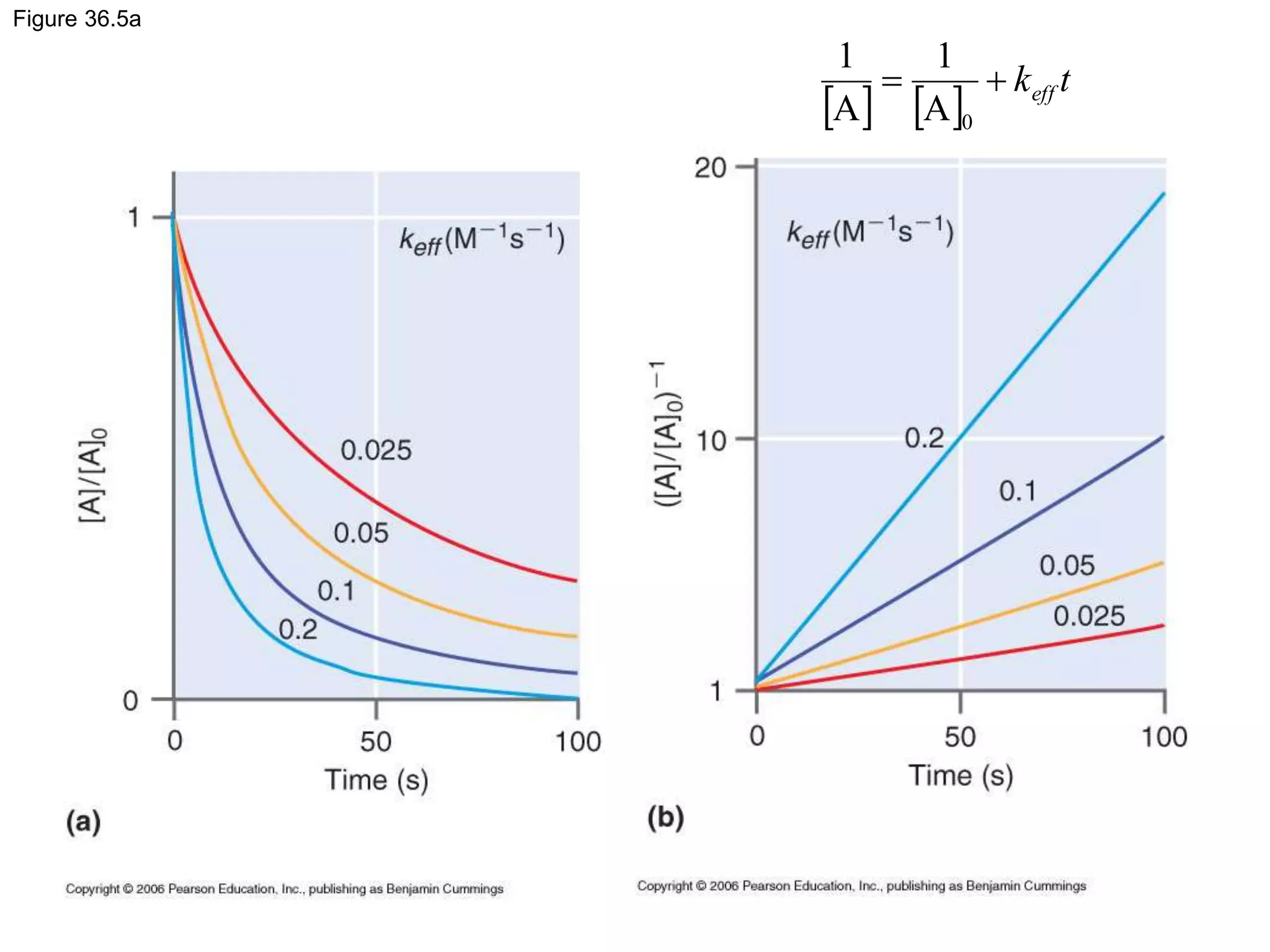
13. 36.5 Integrated Rate Law Expressions
 
 
 
 
 
 
 
    kt
e
e
kt
kdt
d
k
dt
d
dt
d
R
k
R
P
kt
kt
t
k






























0
0
0
0
0
0
A
A
A
ln
A
ln
1
]
A
[
A]
[
]
A
[
]
P
[
A
]
A
[
;
A
A
ln
A
]
A
[
];
A
[
]
A
[
]
A
[
];
A
[
A
reaction
Order
-
First
0

14. 36.5 Integrated Rate Law Expressions
  kt

 0
A
ln
]
A
ln[
 
kt
e

0
A
]
A
[

15. 36.5 Integrated Rate Law Expressions
 
 
k
k
kt
2
ln
2
ln
A
2
/
A
ln
Reaction
Order
-
First
and
life
-
Half
2
/
1
0
0
2
/
1














16. Example 36.3
Example Problem 36.3
The decomposition of N2O5 is an important process in tropospheric
chemistry. The half-life for the first order decomposition of this
compound is 2.05×104 s. How long will it take for a sample of N2O5 to
decay to 60% of its initial value?
Solution
   
       
 
s
10
51
.
1
s
10
38
.
3
6
.
0
ln
6
.
0
O
N
O
N
6
.
0
O
N
O
N
O
N
s
10
38
.
3
s
10
05
.
2
2
ln
2
ln
4
1
-
5
s
10
38
.
3
s
10
38
.
3
0
5
2
0
5
2
5
2
0
5
2
5
2
1
-
5
4
2
/
1
1
-
5
1
-
5























t
e
e
e
t
k
t
t
kt

17. Example 36.3
Example Problem 36.4
Catbon-14 is a radioactive nucleus with half-life of 5760 years. Living
matter exchange carbon with its surroundings (for example, through CO2)
so that s constant level of C14 is maintained, corresponding to 15.3 decay
events per minute. Once living matter has died, carbon contained in the
matter is not exchanged with the surroundings, and the amount of C14
that remains in the dead material decreases with time due to radioactive
decay. Consider a piece of fossilized wood that demonstrates 2.4 C decay
events per minute. How old is the wood.

18. Example 36.4
 
 
 
 
 
    s
10
86
.
4
157
.
0
ln
s
10
81
.
3
1
C
C
ln
1
C
C
157
.
0
min
3
.
15
min
4
.
2
C
C
s
10
81
.
3
s
10
82
.
1
2
ln
years
5760
2
ln
2
ln
11
1
-
12
0
14
14
0
14
14
1
-
1
-
0
14
14
1
-
12
11
2
/
1




























k
t
e
t
k
kt
Solution

19. 36.5 Integrated Rate Law Expressions
 
 
 
   
t
k
dt
k
d
k
dt
d
dt
d
R
k
R
P
eff
t
eff
k














0
0
A
A
2
2
2
A
1
A
1
A
]
A
[
;
]
A
[
2
]
A
[
]
A
[
2
1
;
]
A
[
A
2
I)
(Type
reaction
Order
-
Second
0

20. Figure 36.5a
   
t
keff


0
A
1
A
1

21. 36.5 Integrated Rate Law Expressions
     
 0
2
/
1
2
/
1
0
2
/
1
0
A
1
A
1
;
A
1
A
2
I)
(Type
Reaction
Order
-
Second
and
life
-
Half
eff
eff
eff
k
k
t
k
t
k





22. 36.5 Integrated Rate Law Expressions
 
       
           
   
A
B
A
B
let
;
A
A
B
B
B
B
A
A
]
B
[
]
A
[
;
B
]
A
[
B
A
II)
(Type
reaction
Order
-
Second
0
0
0
0
0
0




















dt
d
dt
d
R
k
R
P
k

23.  
 
 
 
 
 
   
kt
kt
kt
kt
kdt
d
k
k
dt
d
t
















































 









 












 















0
0
0
0
0
0
0
0
A
A
0
A
A
]
A
/[
]
A
[
]
B
/[
]
B
[
ln
A
B
1
]
B
[
]
B
[
ln
]
A
[
]
B
[
ln
1
]
A
[
]
A
[
ln
]
A
[
]
A
[
ln
1
]
A
[
]
A
[
ln
1
]
A
[
]
A
[
]
A
[
]
A
[
]
A
[
]
B
][
A
[
]
A
[
0
0
36.5 Integrated Rate Law Expressions

24. Figure 36.6
   
       
         t
t
t
t
t
k
t
k
k
t
k
t
k
dt
d
A
A
A
A
A
A
A
;
A
A
A
A
P
A




















Figure 36.6
Schematic representation of the
numerical evaluation of a rate law.

25. Figure 36.7
Figure 36.7
Comparison of the numerical approximation
method to the integrated rate law expression
for a first-order reaction. The rate constant
for the reaction is 0.1 m s-1. The time
evolution in reactant concentration
determined by the integrated rate law
expression

26. 36.7 Sequential First-Order Reaction
   
     
   
I
P
I
A
I
A
A
P
I
A
I
I
A
A
I
A
k
dt
d
k
k
dt
d
k
dt
d
k
k










At t = 0
   
         
    
       
       
   0
A
I
A
0
0
0
A
I
A
0
A
A
0
A
1
P
I
A
A
P
P
I
A
A
A
I
I
A
I
A
I
A
A
I
A
A
A
































k
k
e
k
e
k
e
e
k
k
k
k
e
k
k
k
dt
d
e
t
k
I
t
k
t
k
t
k
t
t
k
t
t
k
A
I
Sequential First-Order
Reaction

27. Figure 36.8a
Figure 36.8
Concentration profiles for a
sequential reaction in which the
reactant (A, blue line) from an
intermediate (I, yellow) that
undergoes subsequent decay to
form the product (P, red line)
where (a) kA=2kf =0.1 s-1.

28. Figure 36.8b
Figure 36.8
Concentration profiles for a
sequential reaction in which the
reactant (A, blue line) from an
intermediate (I, yellow) that
undergoes subsequent decay to
form the product (P, red line)
where (b) kA=8kf =0.4 s-1. Notice
that both the maximal amount of I
in a ddition to the time for the
maximum is changed relative to
the first channel.

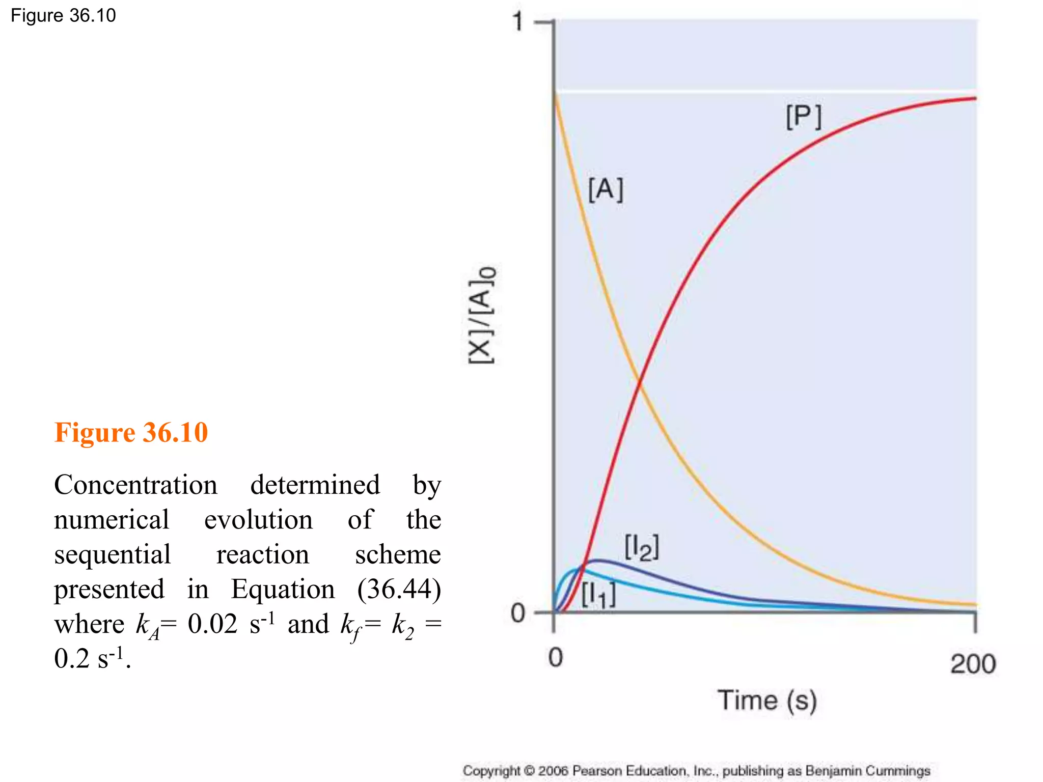
29. Figure 36.8c
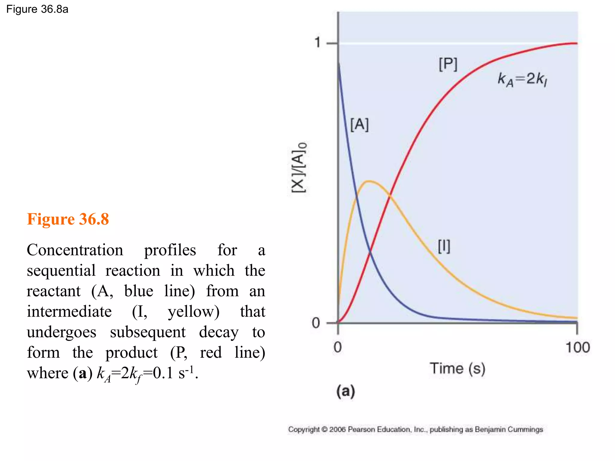
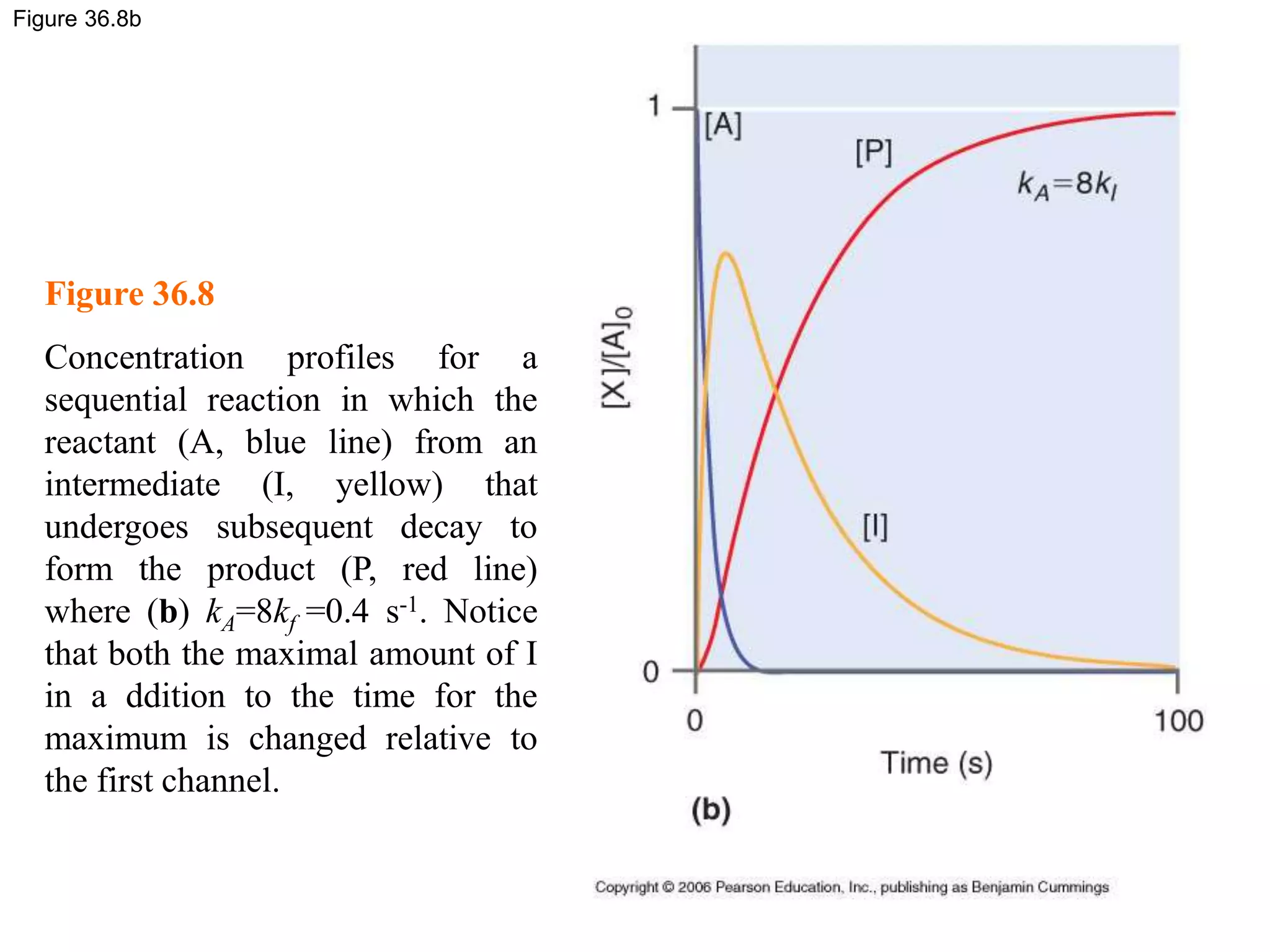
Figure 36.8
Concentration profiles for a
sequential reaction in which the
reactant (A, blue line) from an
intermediate (I, yellow) that
undergoes subsequent decay to
form the product (P, red line)
where (c) kA=0.025kf=0.0125 s-1.
In this case, very little
intermediate is formed, and the
maximum in [I] is delayed relative
to the first two examples.

30. 36.7 Sequential First-order Reaction
Maximum Intermediate Concentration
 


















I
A
I
A
t
t
k
k
k
k
t
dt
d
ln
1
0
I
max
max

31. Example problem 36.5
Example Problem 36.5
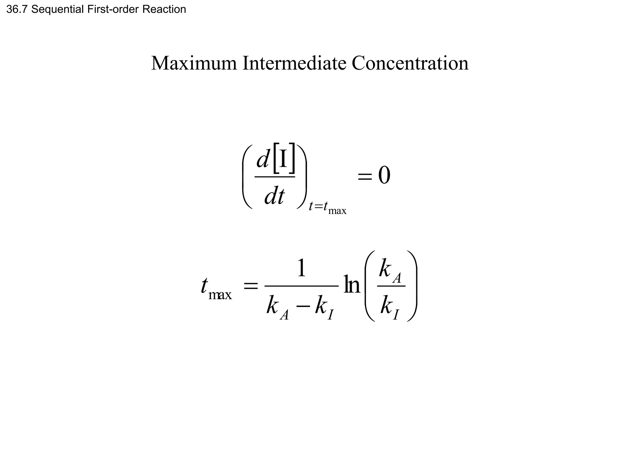
Determine the time at which [I] is at a maximum for
kA = 2kI = 0.1 s-1.
Solution
s
9
.
13
s
05
.
0
s
1
.
0
ln
s
05
.
0
s
1
.
0
1
ln
1
1
-
-1
1
-
1
-
max 




















I
A
I
A k
k
k
k
t

32. Rate-Determining Steps
      
      0
0
0
0
A
1
A
1
lim
P
lim
A
1
A
1
lim
P
lim
t
k
A
I
t
k
I
t
k
A
k
k
t
k
t
k
I
A
t
k
A
I
t
k
I
t
k
A
k
k
t
k
t
k
I
A
IA
A
I
A
A
I
A
I
A
I
A
A
I
A
e
k
k
e
k
e
k
e
e
k
k
e
k
k
e
k
e
k
e
e
k
k




































































36.7 Sequential First-order Reaction

33. Figure 36.9a
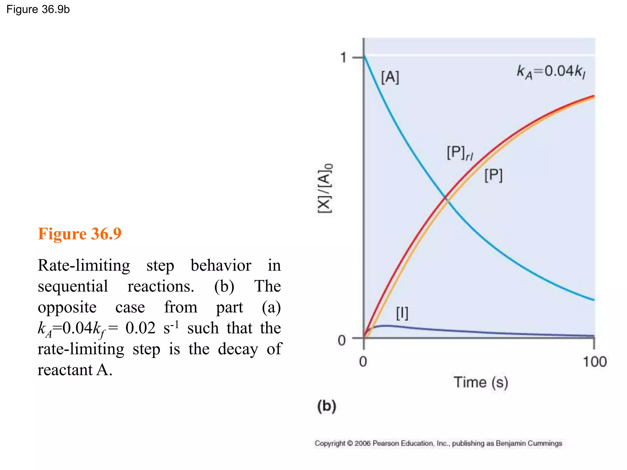
Figure 36.9
Rate-limiting step behavior in
sequential reactions. (a) kA=20kf
=1 s-1 such that the rate-limiting
step is the decay of intermediate I.
In this case, the reduction in [I] is
reflected by the appearances of [P].
The time evolution of [P]
predicted by the sequential
mechanism is given by the yellow
line, and the corresponding
evolution assuming rate-limiting
step behavior, [P]rl, is given by the
red curve.

34. Figure 36.9b
Figure 36.9
Rate-limiting step behavior in
sequential reactions. (b) The
opposite case from part (a)
kA=0.04kf = 0.02 s-1 such that the
rate-limiting step is the decay of
reactant A.

35. 36.7 Sequential First-order Reaction
   
     
     
   
2
2
2
2
1
1
2
1
1
1
2
1
P
A
A
A
P
A 2
1
A
I
k
dt
d
I
k
I
k
dt
I
d
I
k
k
dt
I
d
k
dt
d
I
I
A
A
k
k
k













The steady-State Approximation
This approximation is particularly god when the decay rate of the
intermediate is greater than the rate of production so that the
intermediates are present at very small concentrations during the
reaction.
In Steady-State approximation, the time
derivative of intermediate concentrations is se
to zero.
           
           
           
t
k
ss
t
k
A
ss
t
k
A
ss
ss
ss
ss
ss
t
k
A
A
ss
ss
A
ss
A
A
A
A
e
e
k
I
k
dt
d
e
k
k
k
k
I
I
k
I
k
dt
I
d
e
k
k
k
k
I
I
k
k
dt
I
d





















1
A
P
A
P
A
I
0
A
A
A
0
0
0
2
2
0
2
1
2
1
2
2
2
1
1
2
0
1
1
1
1
1
1

36. Figure 36.10
Figure 36.10
Concentration determined by
numerical evolution of the
sequential reaction scheme
presented in Equation (36.44)
where kA= 0.02 s-1 and kf = k2 =
0.2 s-1.

37. Figure 36.11
Figure 36.11
Comparison of the numerical and
steady-state concentration profiles
for the sequential reaction scheme
presented in Equation (36.44) where
kA= 0.02 s-1 and kf = k2 = 0.2 s-1.
Curves corresponding to the steady-
state approximation are indicated by
the subscript ss.

38. 36.8 Parallel Reactions
Parallel Reactions         
       
     
     
     
 
     
 
 
  A
B
t
k
k
C
B
C
t
k
k
C
B
B
t
k
k
C
B
C
B
C
B
k
k
e
k
k
k
e
k
k
k
e
condition
initial
k
dt
d
k
dt
d
k
k
k
k
dt
d
C
B
C
B
C
B


























C
B
1
A
C
1
A
B
A
A
0
C
B
,
0
A
C
C
;
A
A
A
A
A
A
0
0
0
0

39. Figure 36.12
Figure 36.12
Concentration for a parallel
reaction where kB = 2kC = 0.1 s-1.

40. 36.8 Parallel Reactions
Yield, F, is defined as the probability that given product
will be formed by decay of the reactant.


F
n
n
i
k
k

41. Example Problem 36.7
In acidic conditions, benzyl peniciline (BP) undergoes the
following paralll reaction:
In the molecular structure, R1 and R2 indicate alkyl substitutions.
In a solution where pH=3, the rat constants for the processes at
22 ℃are k1=7.0×10-4 s-1, k2=4.1×10-3 s-1, and k2=5.7×10-3 s-1.
what is the yield for P1 formation?
Example Problem 36.7

42. Example Problem 36.7
067
.
0
s
10
7
.
5
s
10
1
.
4
s
10
0
.
7
s
10
0
.
7
1
3
1
3
1
4
1
4
3
2
1
1
P1











F 







k
k
k
k
Solution

43. 36.9 Temperature Dependence of Rate Constants
RT
E
A
k
Ae
k
rrehenius
a
RT
Ea


 
ln
ln
expression
A
/
A frequency factor or Arrhenius pre-exponential factor
Ea activation energy

44. Example Problem 36.8
Example Problem 36.8
The temperature dependence of the acid-catalyzed hydrolysis of
penicillin (illustrated in Example problem 36.7) is investigated,
and the dependece of k1 on temperature is iven in the following
table. What is the activation eergy and Arrhenius preexponential
factor for this branch of hydrolysis reaction?
Temperature ℃ k1 （s-1）
22.2 7.0×10-4
27.2 9.8×10-4
33.7 1.6×10-3
38.0 2.0×10-3

45. Example Problem 36.8
Draw a plot of ln (k1) versus 1/T
   
1
1
-
1
6
1
.
14
mole
K
J
314
.
8
K
3
.
6306
10
33
.
1
1
.
14
ln
1
.
14
T
1
K
3
.
6306
ln















a
a
E
R
E
slope
s
e
A
A
k
Solution

46. 36.9 Temperature Dependence of Rate Constant
Figure 36.13 A schematic drawing of the energy profile for a
chemical reaction. Reactants must acquire sufficient energy to
overcome the activation energy, Ea, for the reaction. The reaction
coordinate represents the binding and geometry changes hat
occur in the transformation of reactants into products.

47. 36.10 Reversible Reactions and Equilibrium
     
     
     
           
 
    
 
    
 
 

 














t
k
k
dt
k
k
k
d
k
k
k
k
-k
k
-k
dt
d
k
-
k
dt
d
k
-k
dt
d
0
A
A 0
B
B
A
0
B
B
A
0
B
A
B
A
0
B
A
B
A
-
A
-
A
A
A
A
-
A
-
A
A
B
A
A
B
A
A
Since
B
A
B
B
A
A
B
A
0
A
B
   
 
   
 
     
      





































B
A
B
0
eq
B
A
B
0
eq
B
A
A
B
0
B
A
A
B
0
1
A
B
lim
B
A
A
lim
A
1
A
B
A
A
B
A
B
A
k
k
k
k
k
k
k
k
e
k
k
k
k
e
k
k
t
t
t
k
k
t
k
k
Reversible Reactions

48. 36.10 Reversible Reactions and Equilibrium
   
   
 
  C
eq
eq
eq
eq
eq
eq
K
k
k
k
k
dt
d
dt
d







A
B
B
A
0
B
A
B
A
B
A
At equilibrium

49. 36.10 Reversible Reactions and Equilibrium
Figure 36.14 Reaction coordinate demonstrating the activation
energy for reactants to form products, Ea, and the back reaction
in which products form reactants, E’a

50. 36.10 Reversible Reactions and Equilibrium
Figure 36.15
Time-dependent concentrations in
which both forward and back reactions
exist between reactant A and product B.
In this example, kA=2kB=0.06 s-1. Note
that the concentration reach a constant
value at longer times (t > teq) at which
pint the reaction reaches equilibrium.

51. 36.10 Reversible Reactions and Equilibrium
Figure 36.16 Methodology for determining fprward and back rate
constants. The apparent rate constant for reactant dacay is equal to
the sum of forward, kA, and back, kB, rate constnats. The equilibrium
constant is equal to kA / kB. These two measurements provide a
system of two equations and two unknowns that can be readily
evaluated to produce kA, and kB.

52. Example Problem 36.9
Example Problem 36.9
Consider the interconversion of the boat and chair conformation
of cyclohexane:
The reaction is first order in each direction, with a equilibrium
constant of 104. The activation enegy for the conversion of the
chair conformer to the boat conformer is 42 kJ/mol. Assuming an
Arrhenius preexponential factor of 1012 s-1, what is the expected
observed reaction rate constant at 298 K if one were to initiate
this reaction starting with only the boat conformer?

53. Example Problem 36.9
  
1
-
8
1
-
8
4
4
1
-
4
1
-
1
-
1
-
1
-
12
/
B
s
10
34
.
4
s
10
34
.
4
10
10
s
10
34
.
4
K
298
K
mol
J
8.314
mol
J
000
,
42
exp
s
10

















 

 
B
A
app
B
A
B
A
C
RT
E
k
k
k
k
k
k
k
K
Ae
k a
Solution

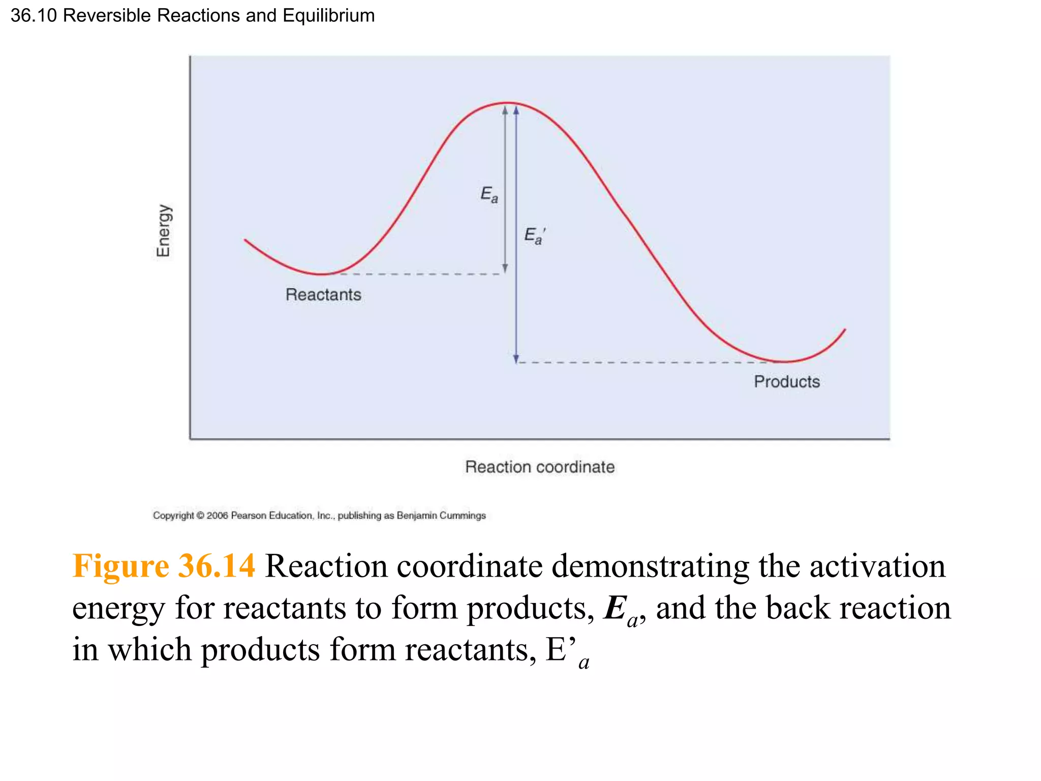
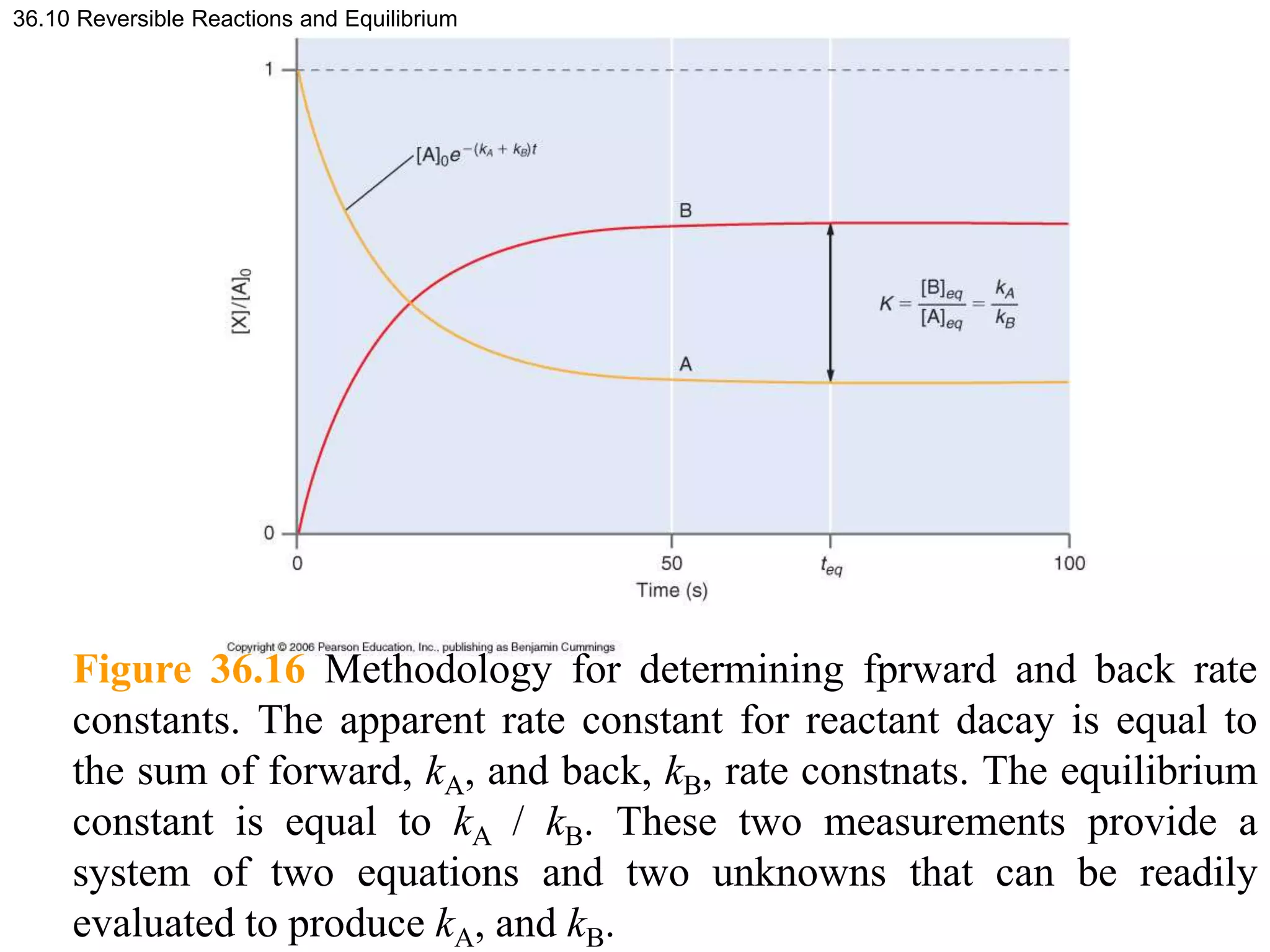
54. Figure 36.17
Figure 36.17 Example of a temperature-jump experiment for a reaction in which
the forward and back rate pocesses are first order. The yellow and blue portions of
the graph indicate times before and after the temperature jump, respectively. After
the temperature jump, [A] decrease with a time constant related to the sum of he
forward and back rate constants. The change between the pre-jump and post-jump
equilibrium concentrations is given by 0

55. 36.13 Potential Energy Surface
Figure 36.18
Definition of geometric coordinates for the AB + CA+BC reaction.

56. 36.13 Potential Energy Surface
Figure 36.19 Illustration of a potential surface for the AB+C reaction at a
colinear geometry (=180° in Figure 36.18). (a,b) Three dimensional views of the
surface.

57. 36.13 Potential Energy Surface
Figure 36.19 Illustration of a
potential surface for the AB+C
reaction at a colinear geometry
(=180° in Figure 36.18). (c) Counter
plot of the surface with contours of
equipotential energy. The curved
dashes line represents the path of a
reactive event, corresponding to the
reaction coordinate. The transition
state for this coordinate is indicated
by the symbol ‡.

58. 36.13 Potential Energy Surface
Figure 36.19 Illustration of a potential surface for the AB+C reaction at a
colinear geometry (=180° in Figure 36.18). (d,e) Cross sections of the potential
energy surface along the lines a-a and b-b, respectively. These two graphs
corresponds to the potential for two-body interactions of B with C, and A with B.

59. Figure 36.20
Figure 36.20 Reaction coordinates involving an activated complex and a
reactive intermediate. The graph corresponds to the reaction coordinate derived
from the dashed line between points c and d on the contour plot of Figure 36.19c.
The maximum in energy along this coordinate corresponds to the transition state,
and the species at this maximum is referred to as an activated complex.

60. Figure 36.21
Figure 36.21
Illustration of transition state theory. Similar to reaction coordinates depicted
previously, the reactants (A and B) and product (P) are separated by an energy
barrier. The transition state is an activated reactant complex envisioned to exist at
the free-energy maximum along the reaction coordinate.