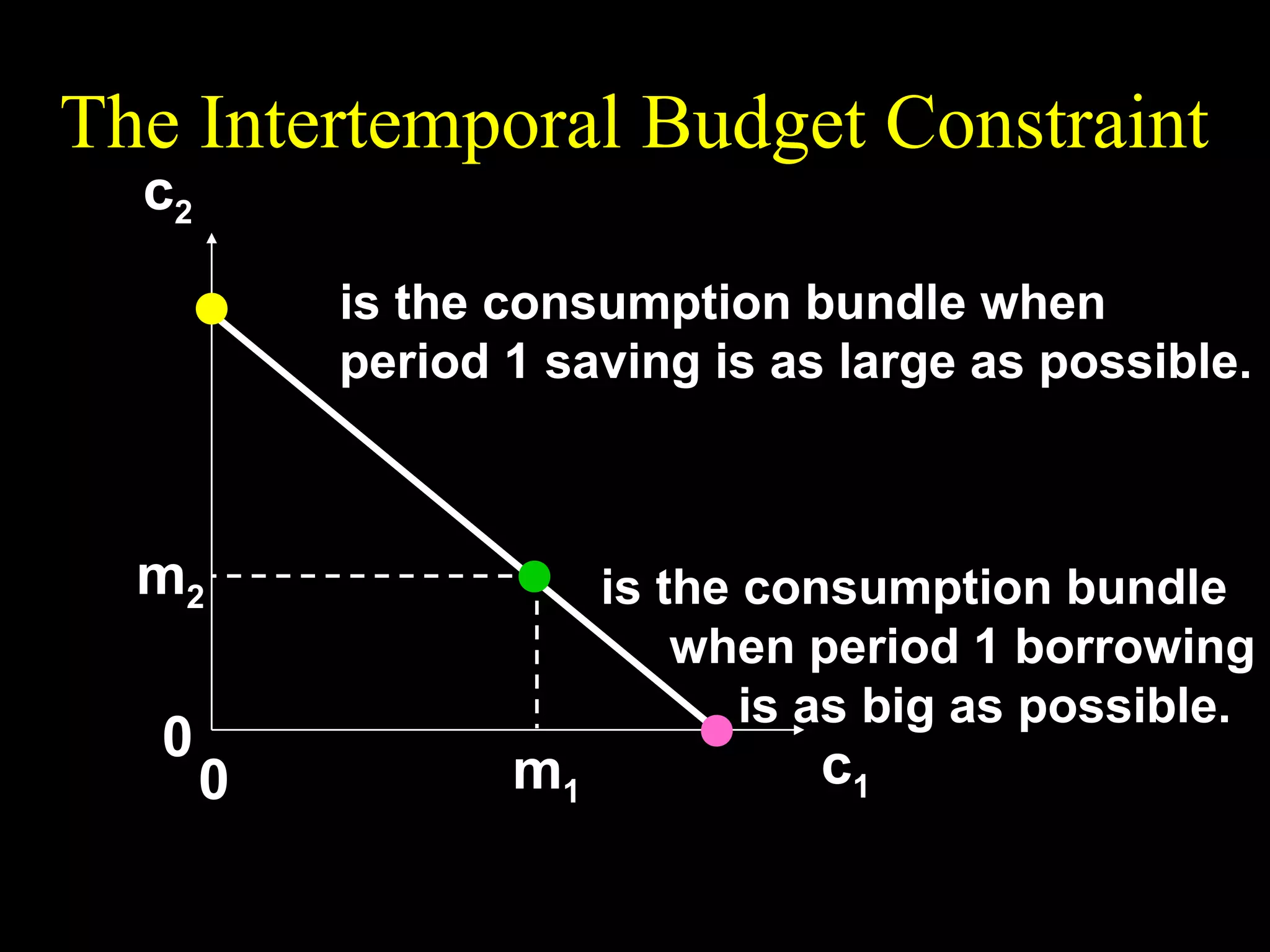
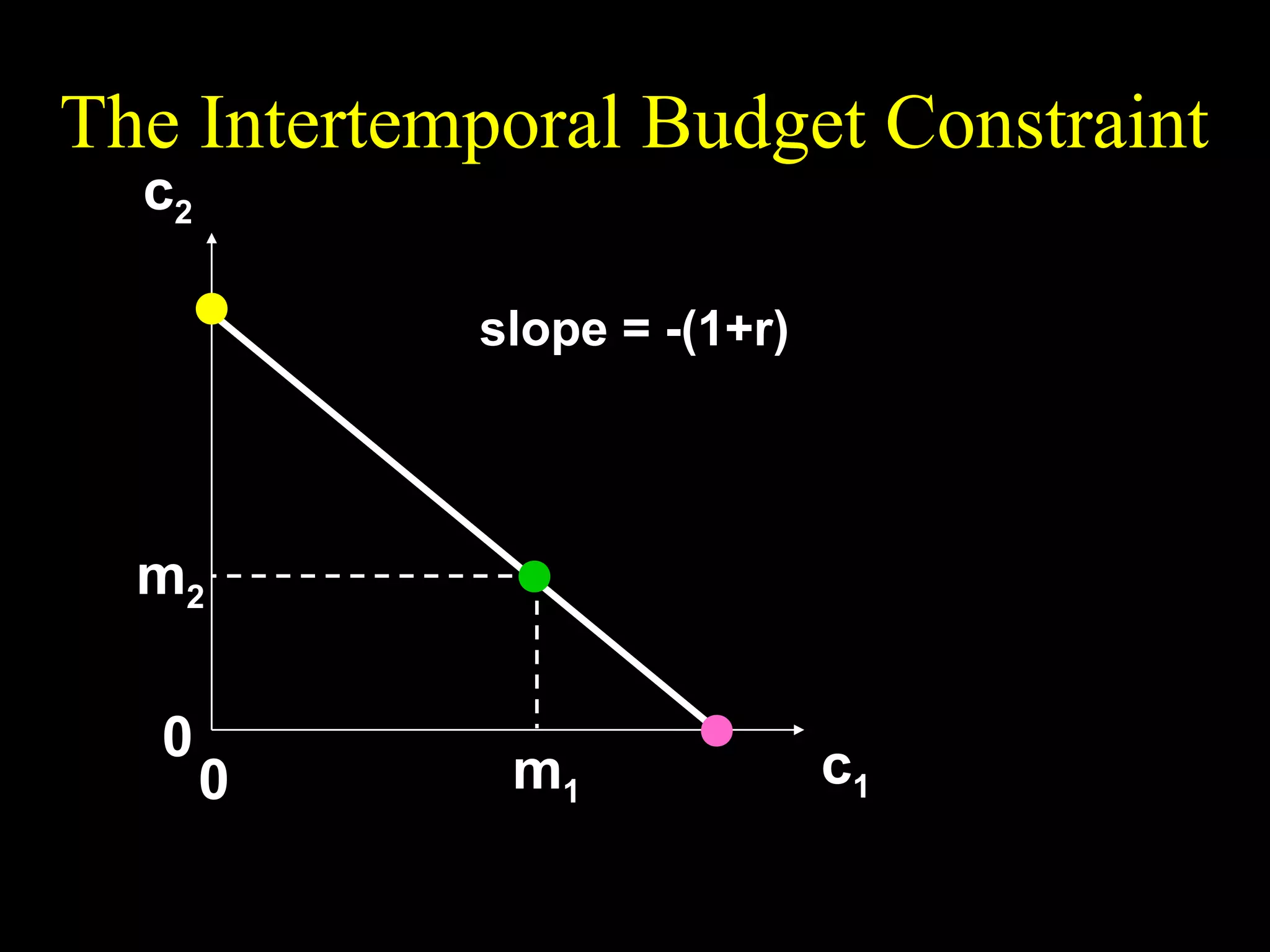
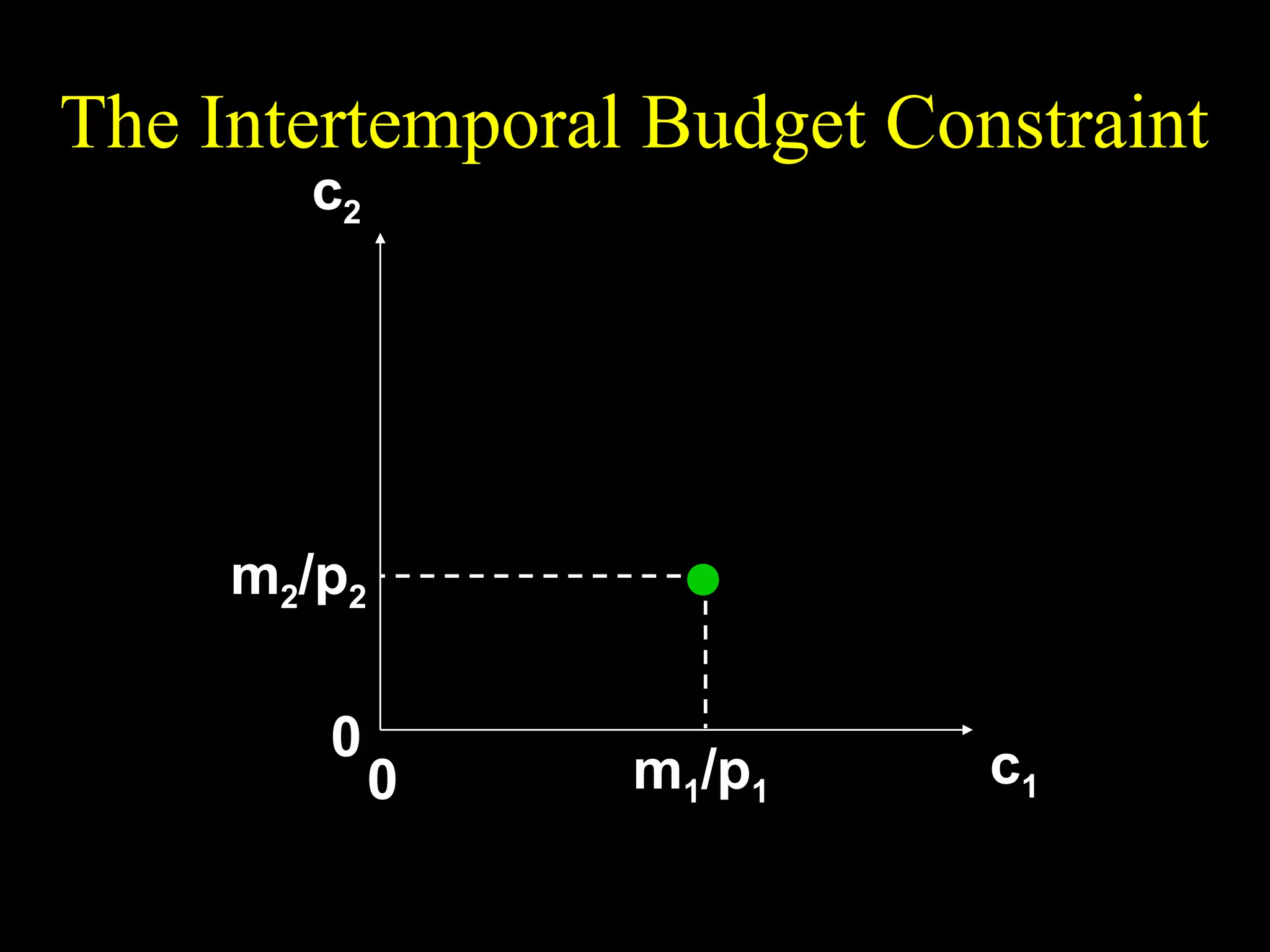
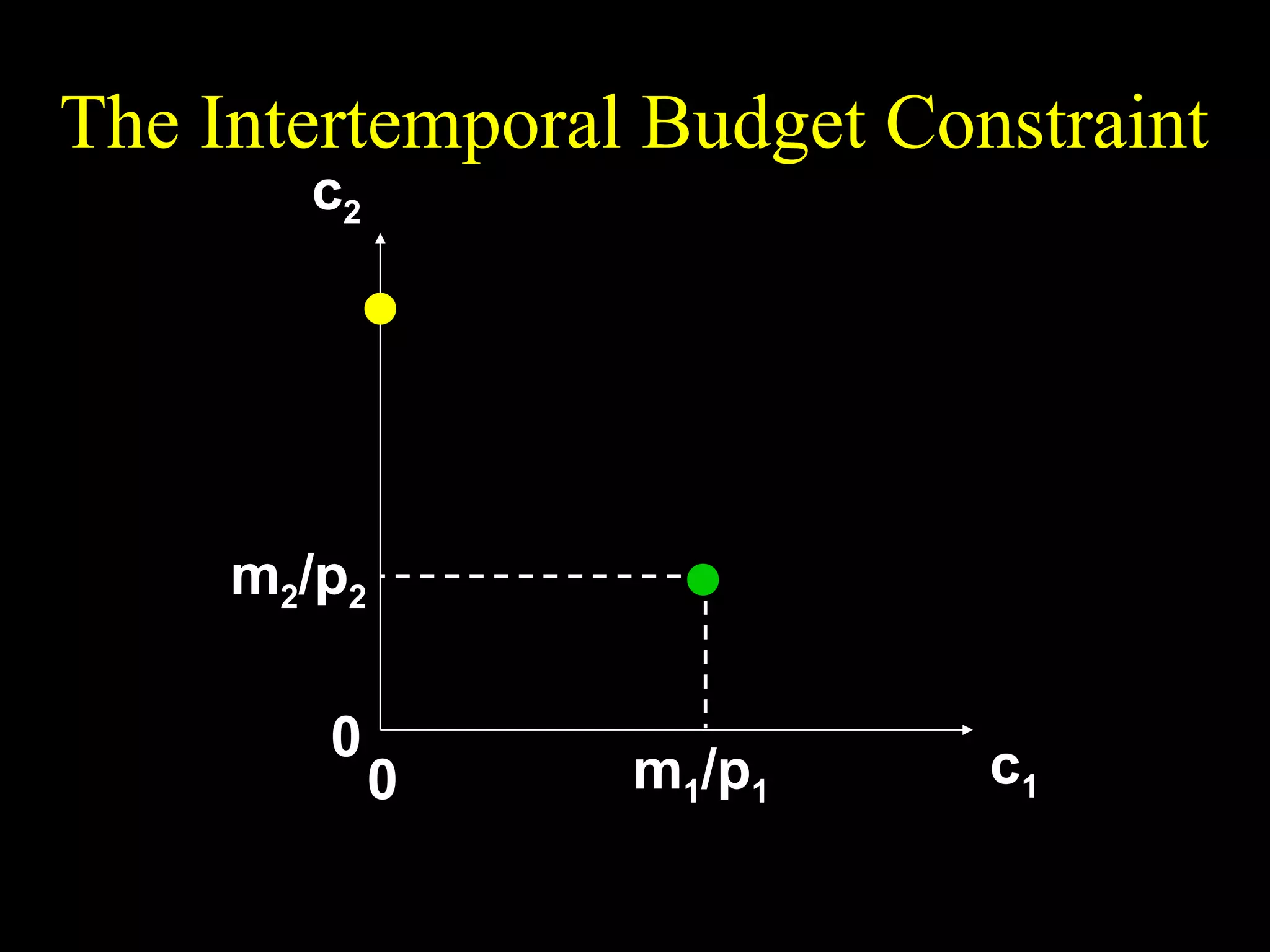
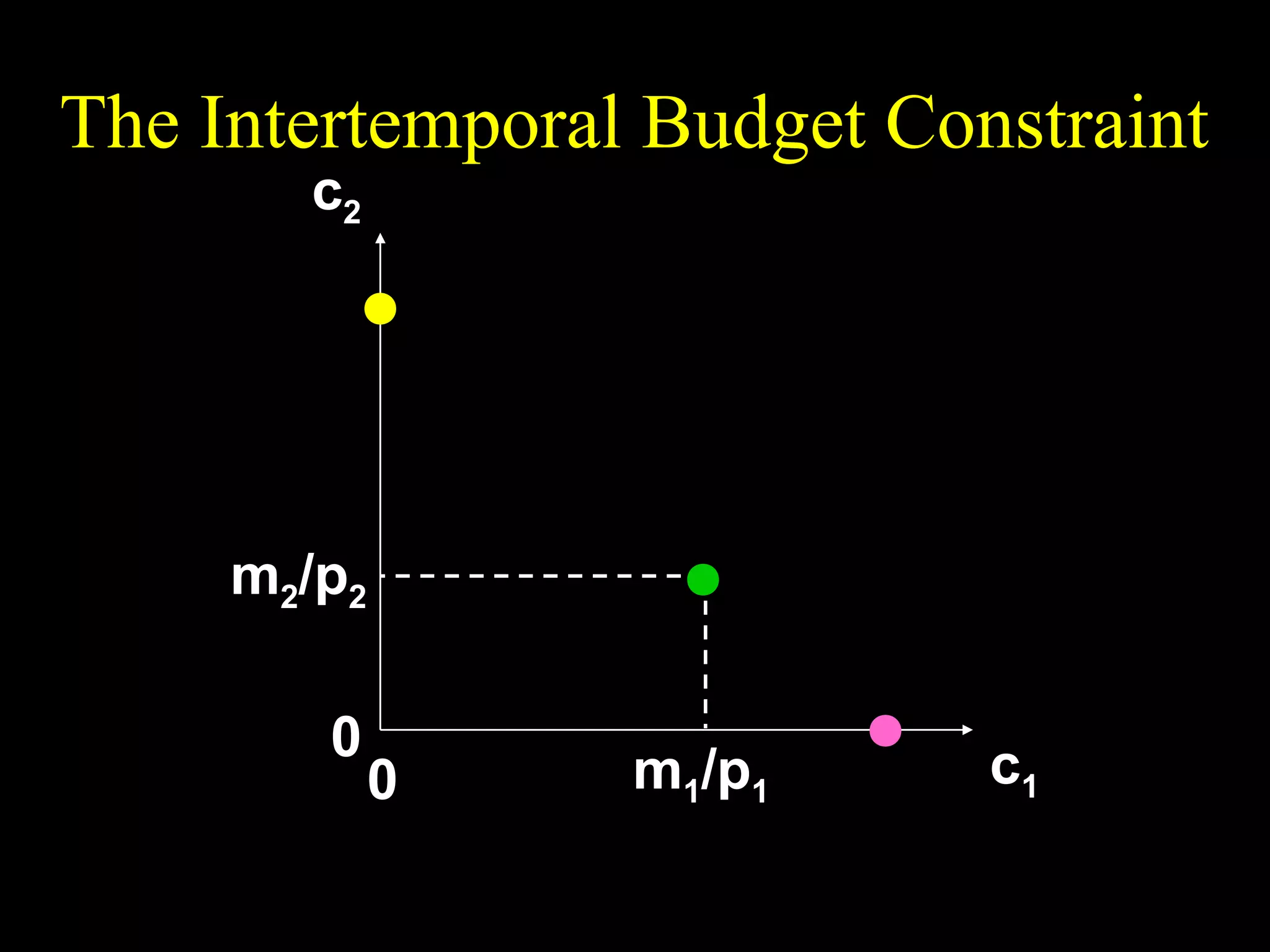
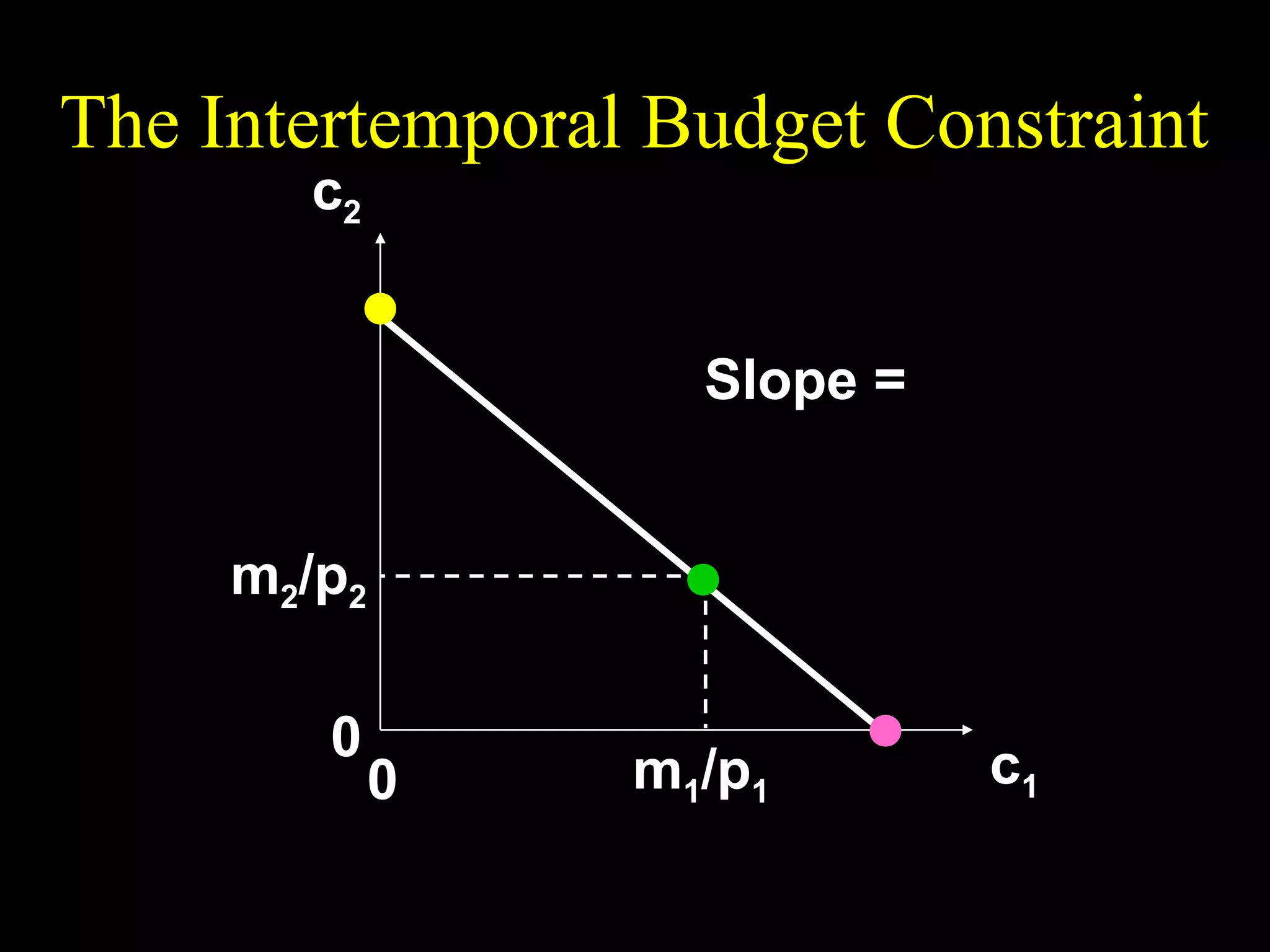
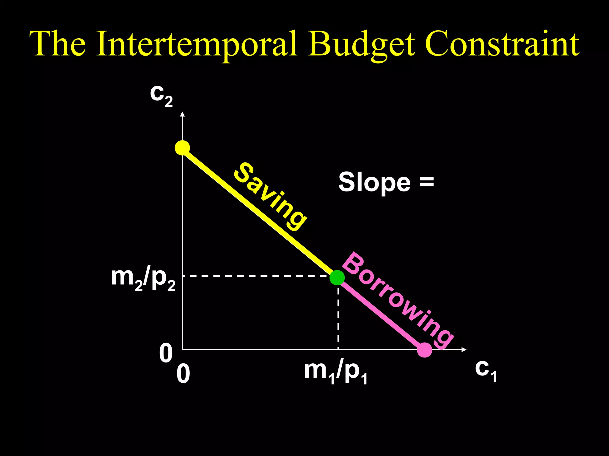
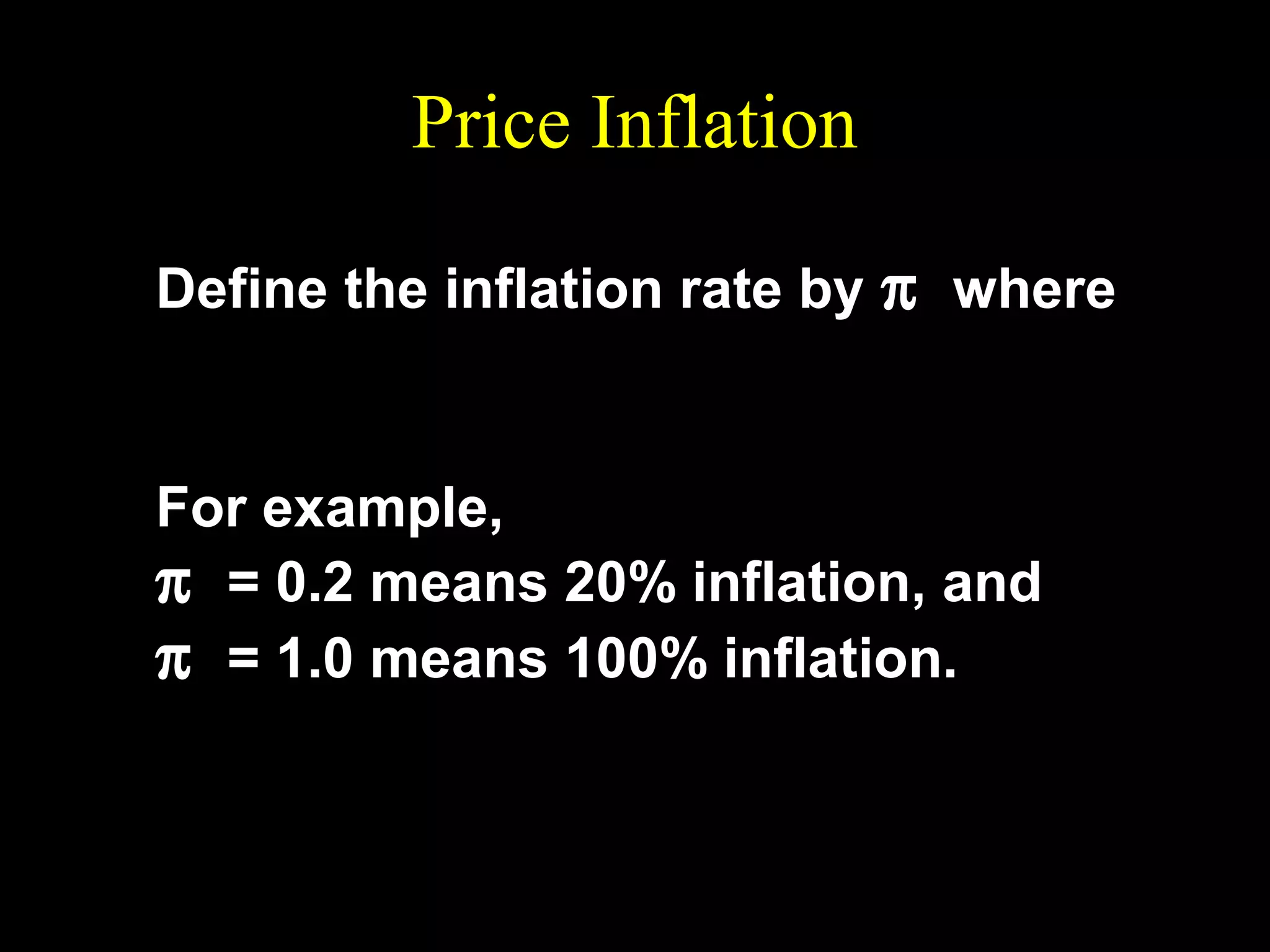
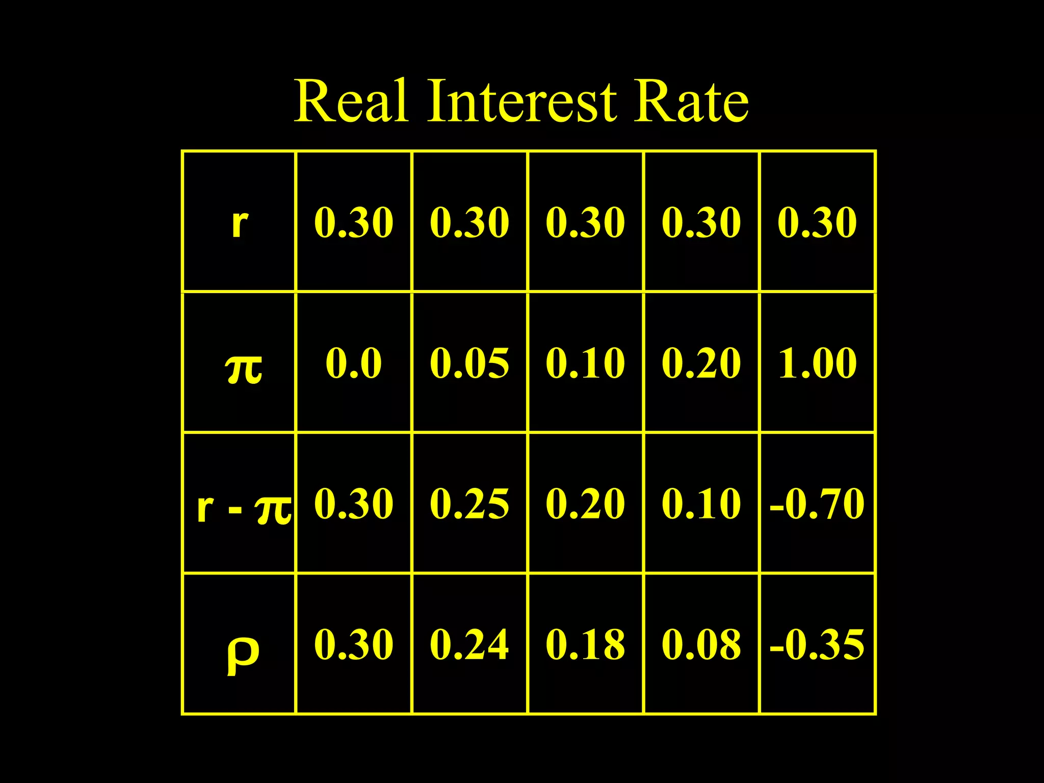
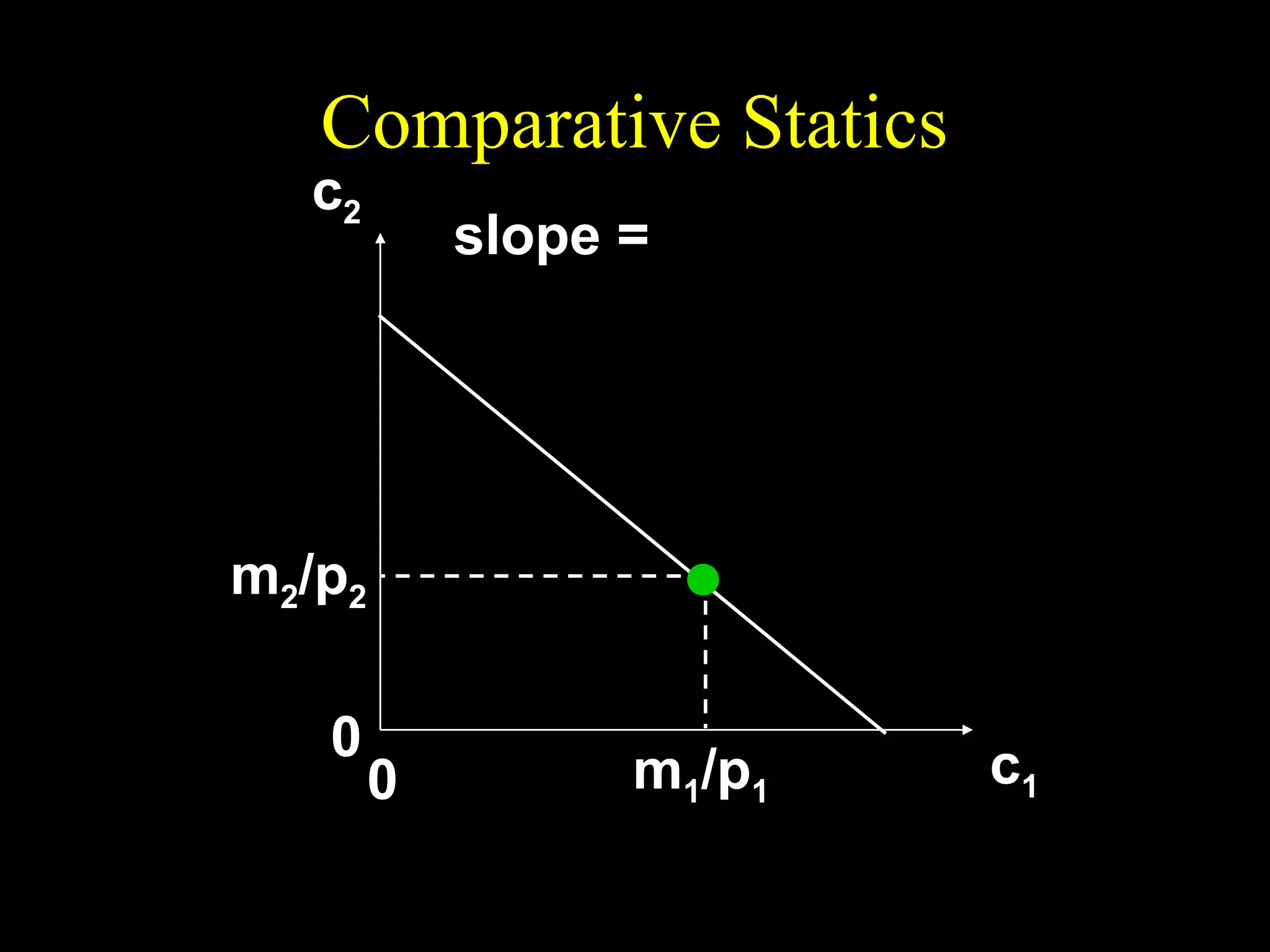
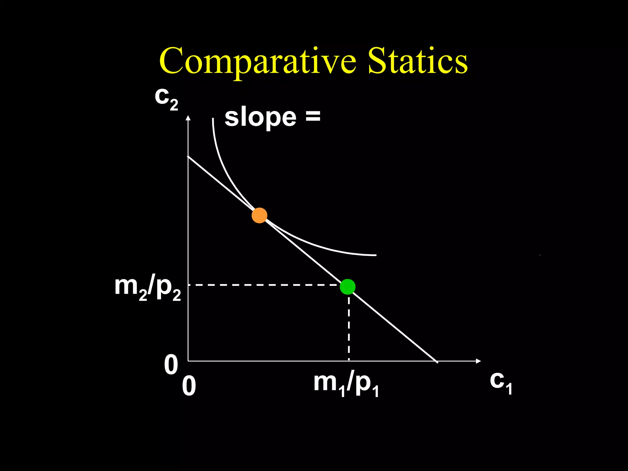
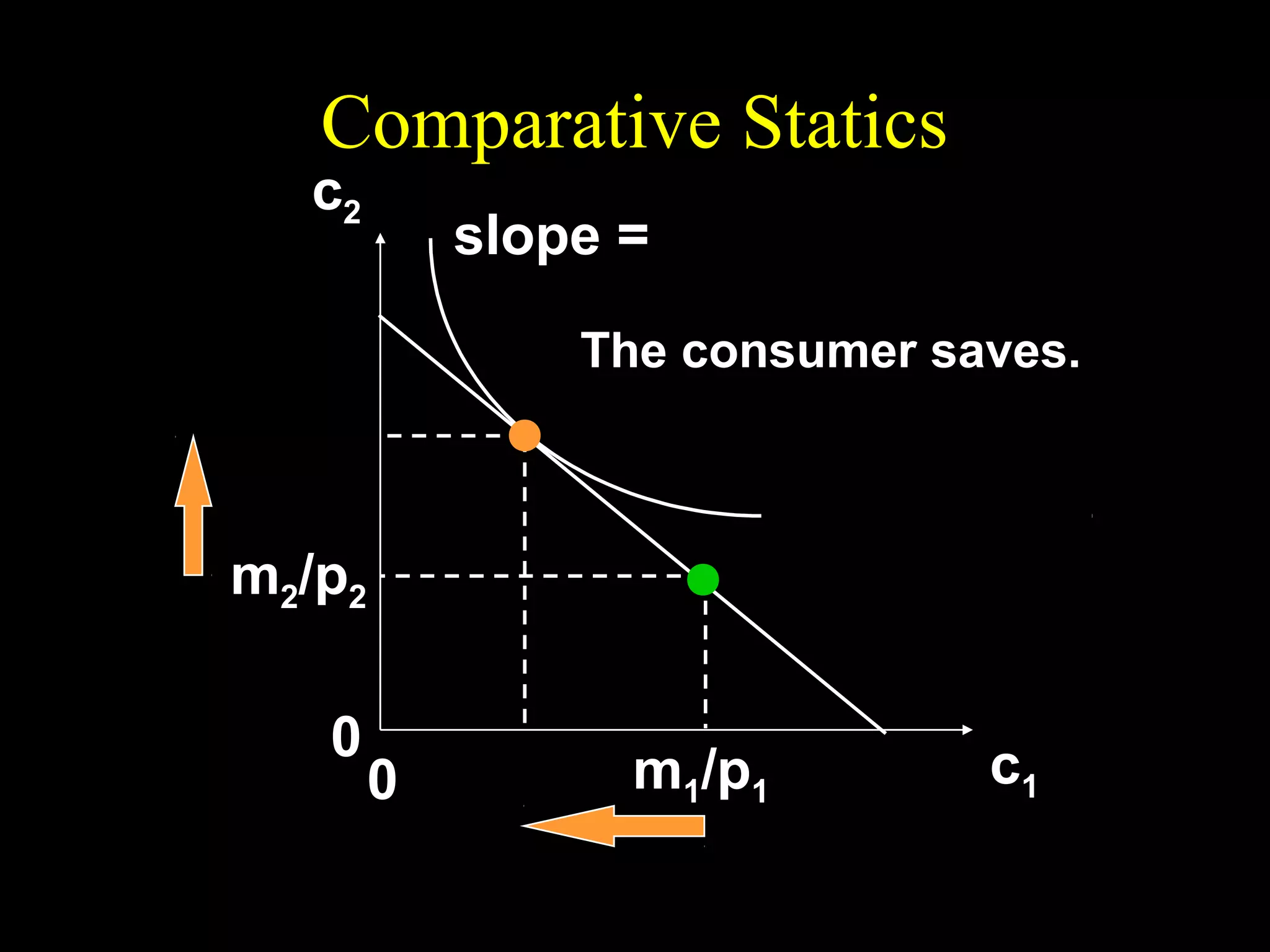
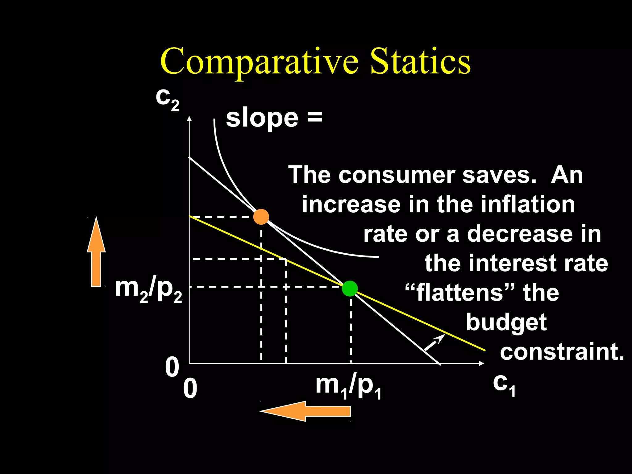
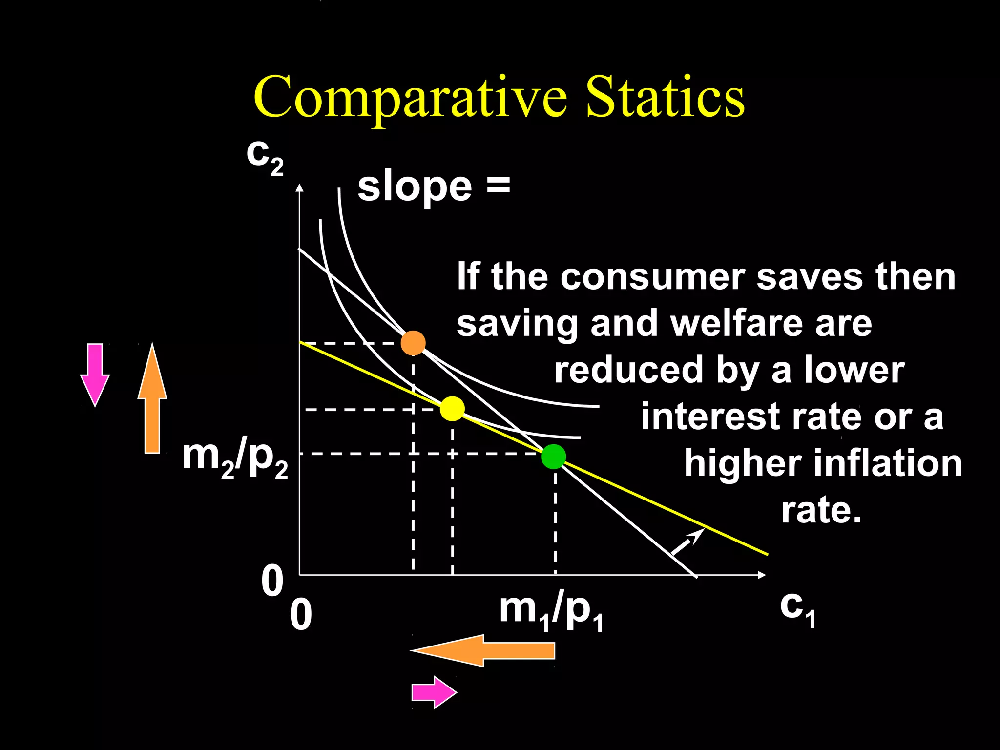
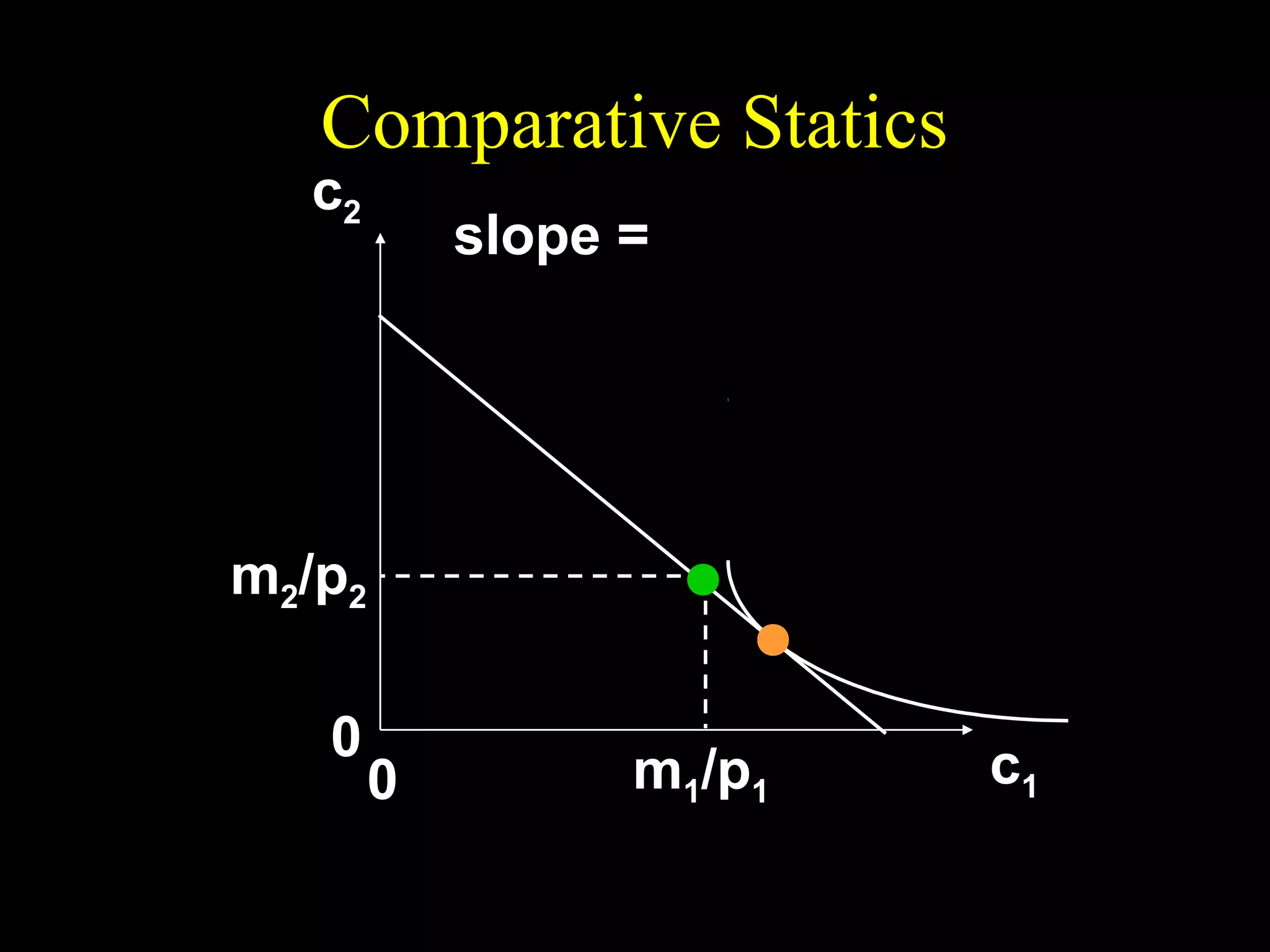
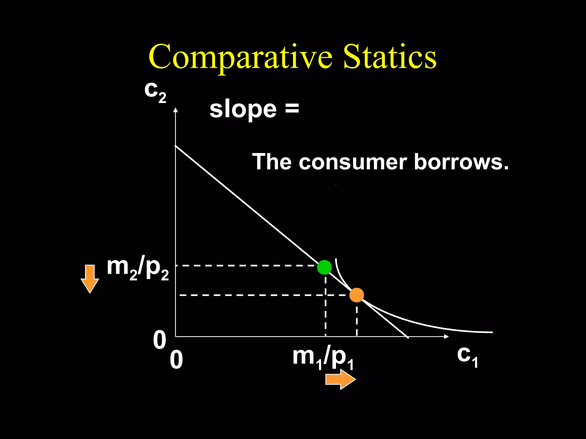
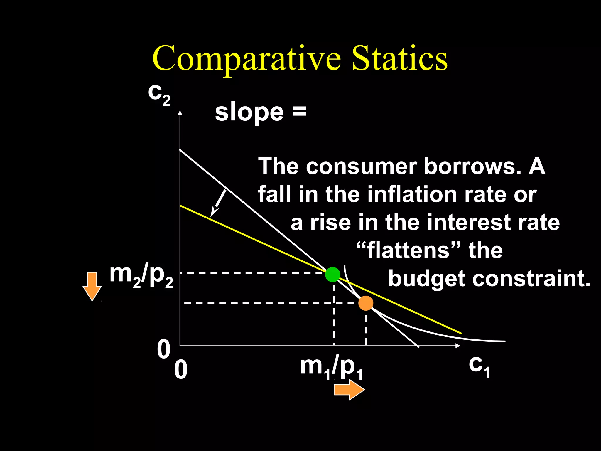
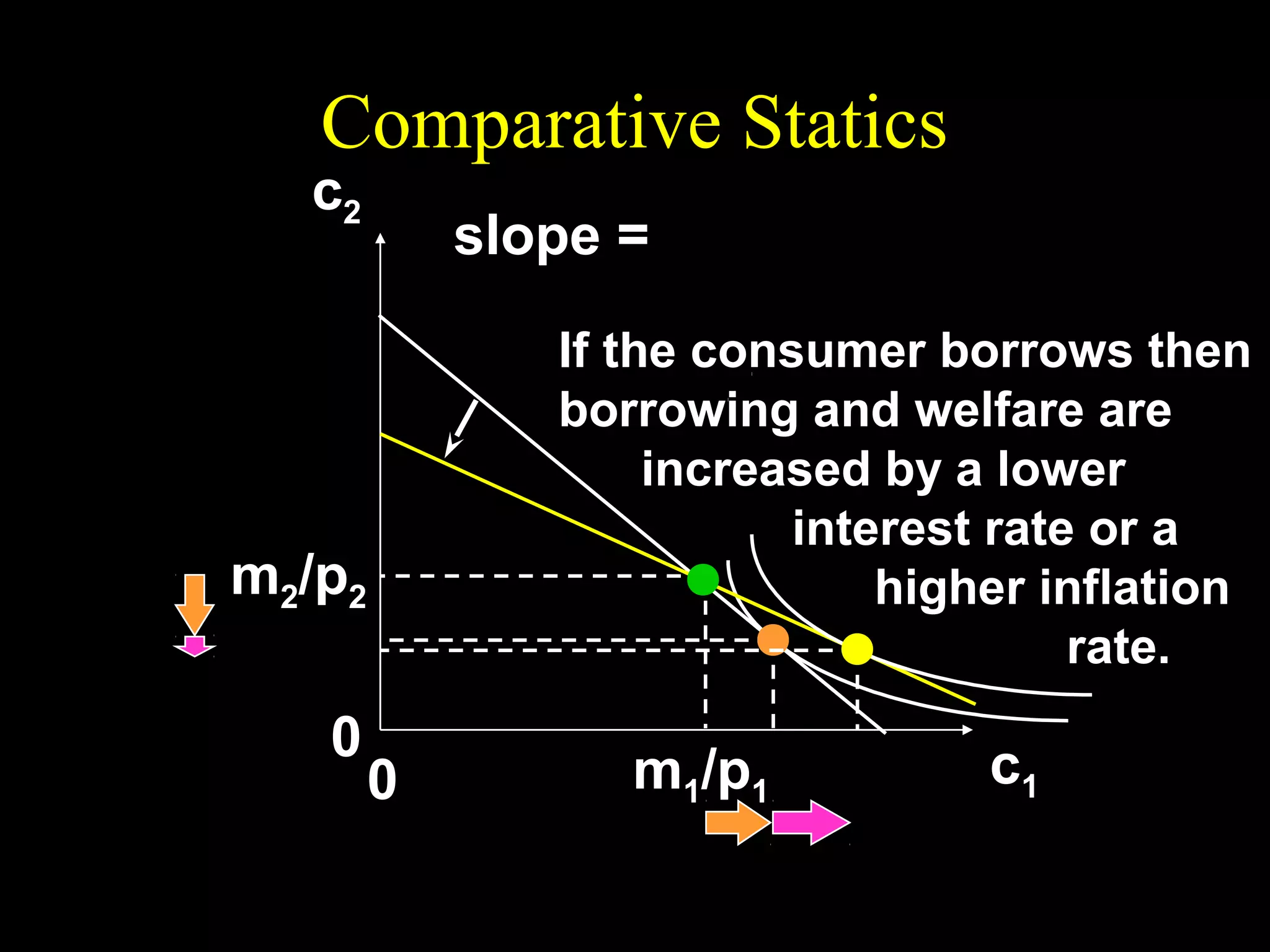
This document discusses intertemporal choice and the intertemporal budget constraint. It begins by introducing the concepts of future value and present value given an interest rate. It then derives the intertemporal budget constraint graphically, showing the consumption bundles when saving, borrowing, or a combination are maximized. Price inflation is incorporated by defining the real interest rate. The slope of the budget constraint depends on the nominal interest rate and inflation. A flatter slope indicates less saving by the consumer.


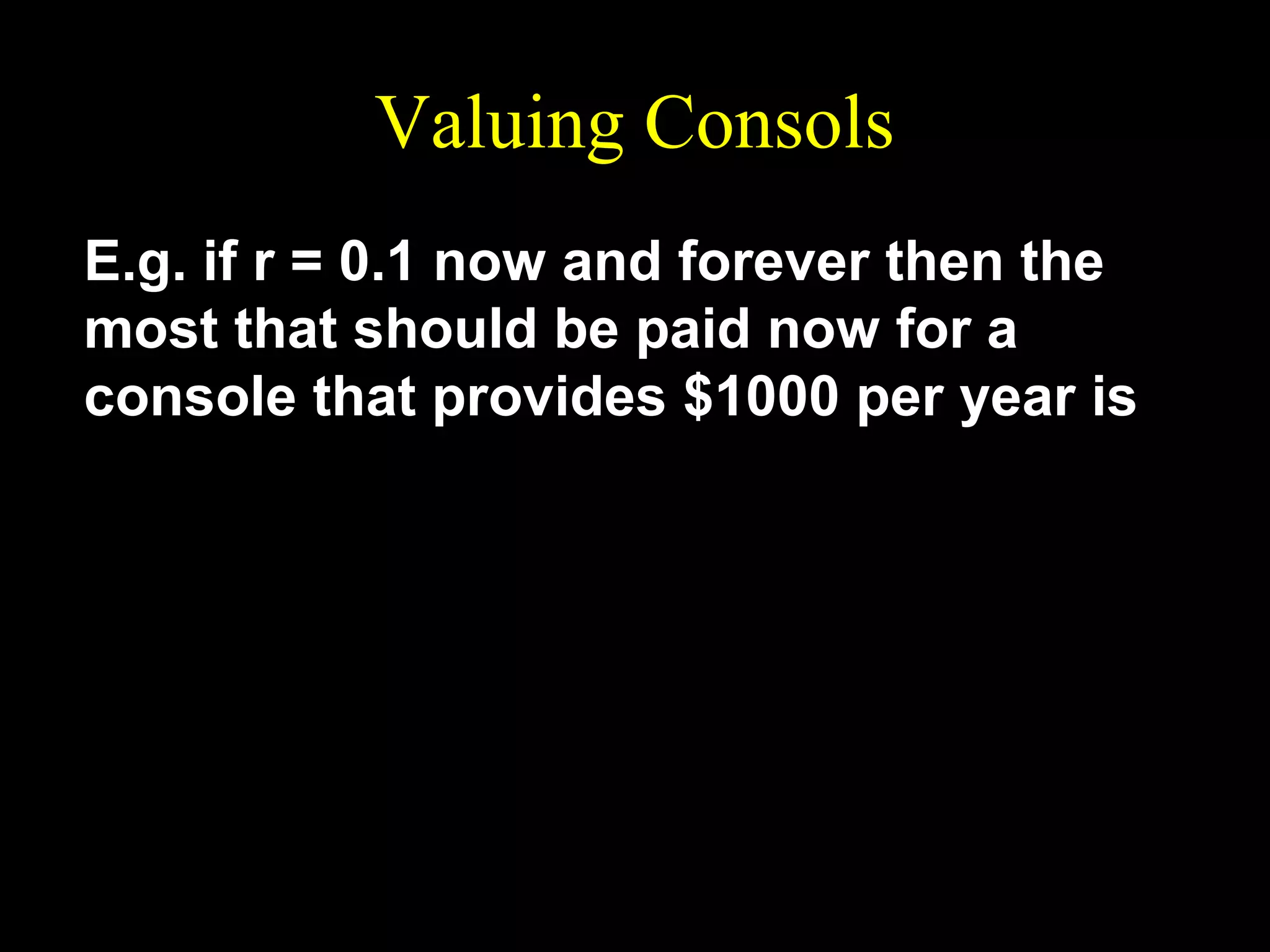
![Valuing Consols
x
x
x
PV =
+
+
+
1 + r (1 + r ) 2 (1 + r ) 3
1
x
x
=
+
+
x +
1+r
1 + r (1 + r ) 2
1
=
[ x + PV] .
1+r
Solving for PV gives
x
PV = .
r](https://image.slidesharecdn.com/ch10-140131134426-phpapp01/75/Ch10-68-2048.jpg)