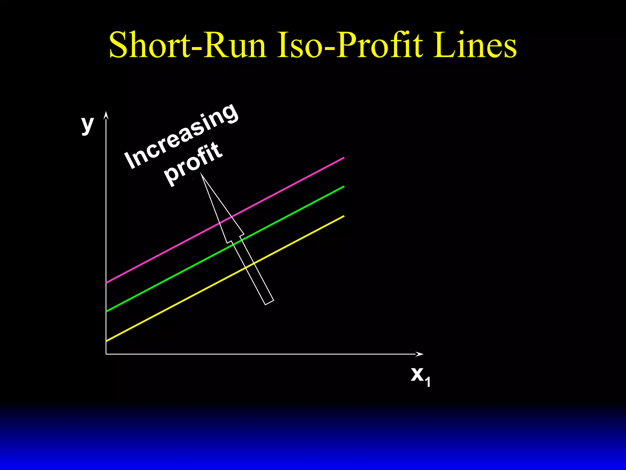
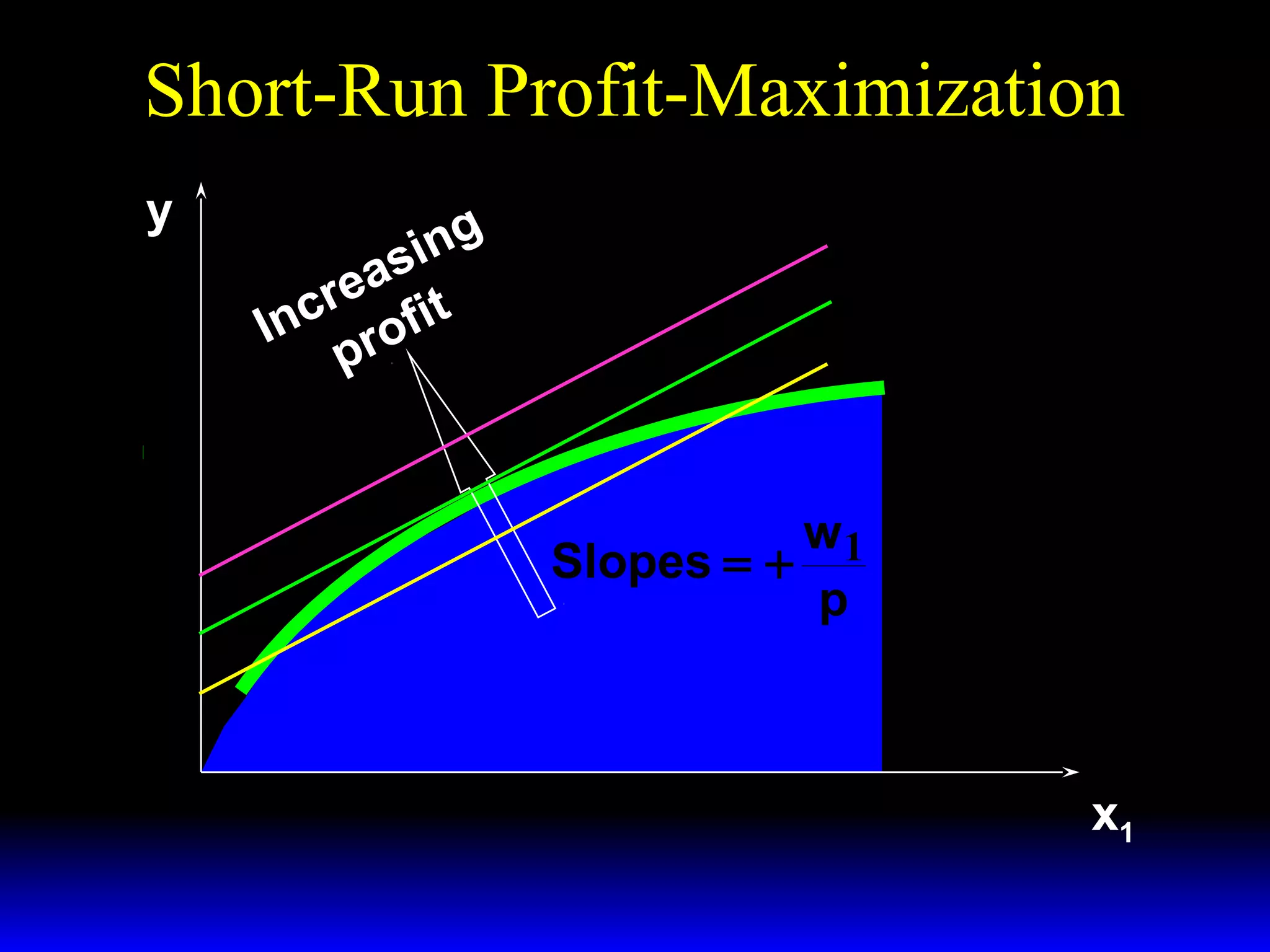
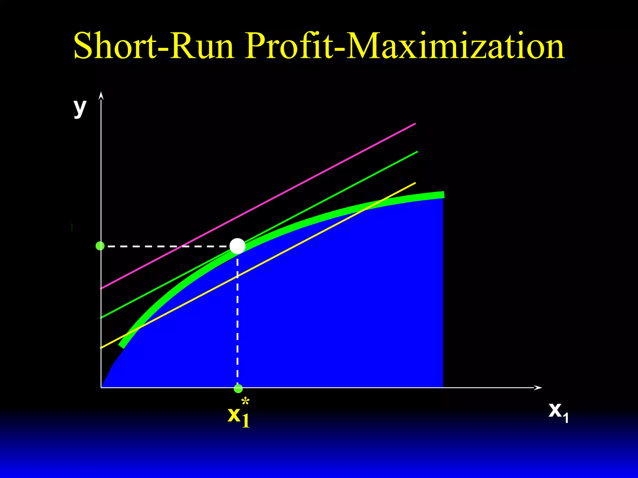
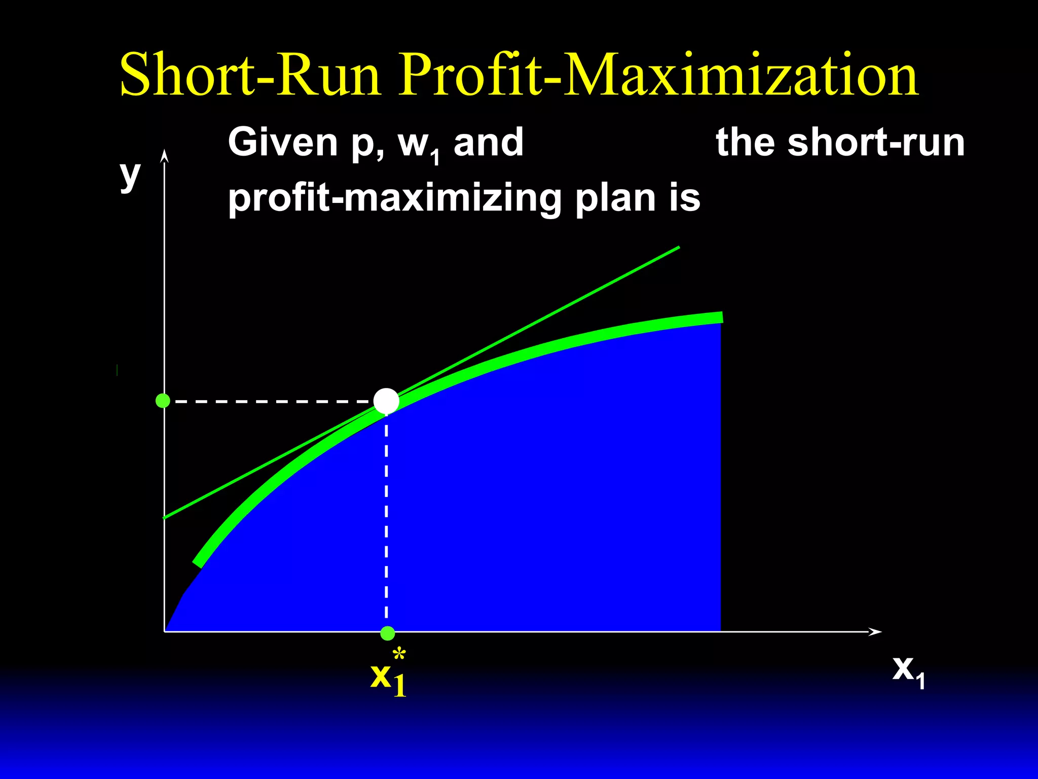
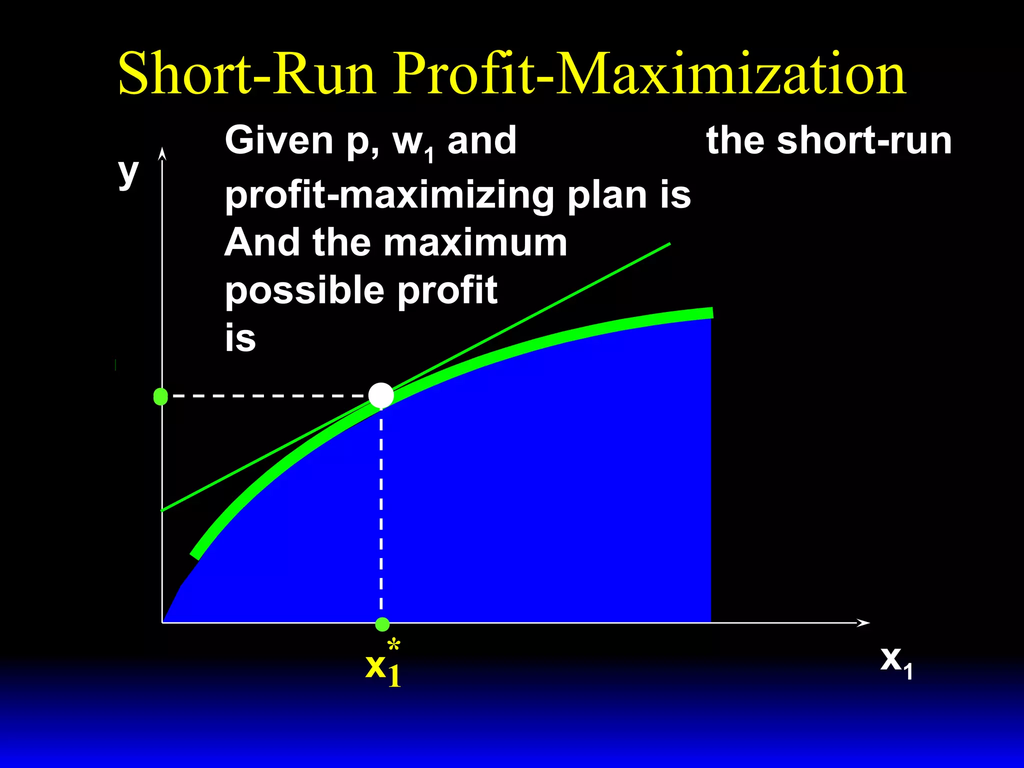
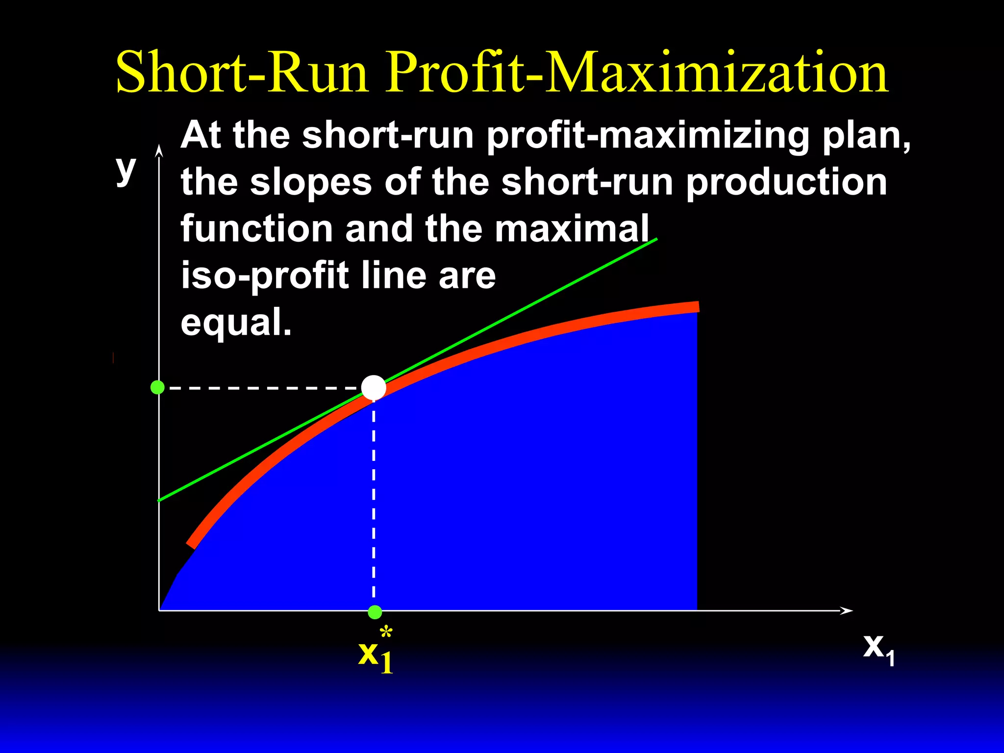
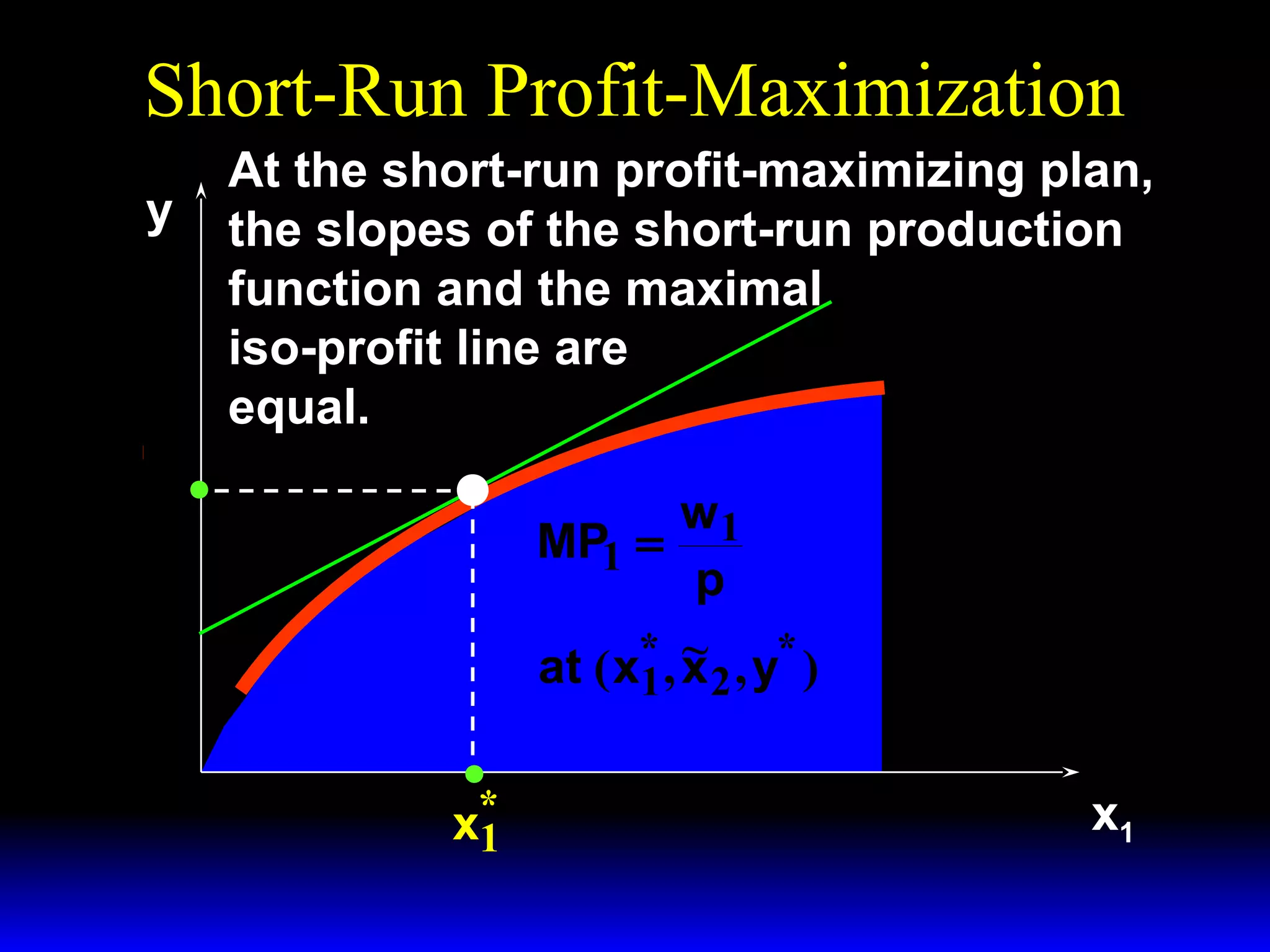
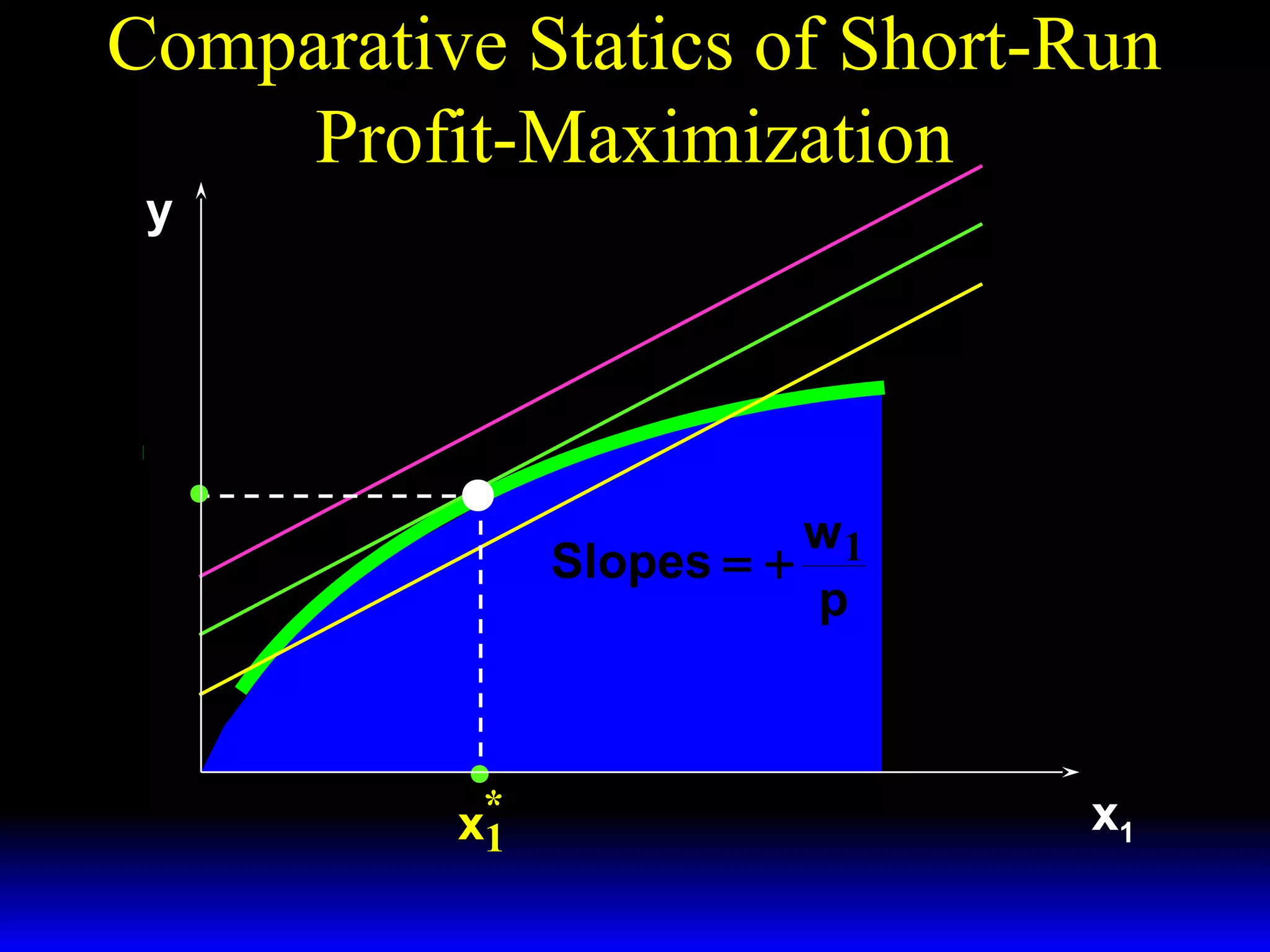
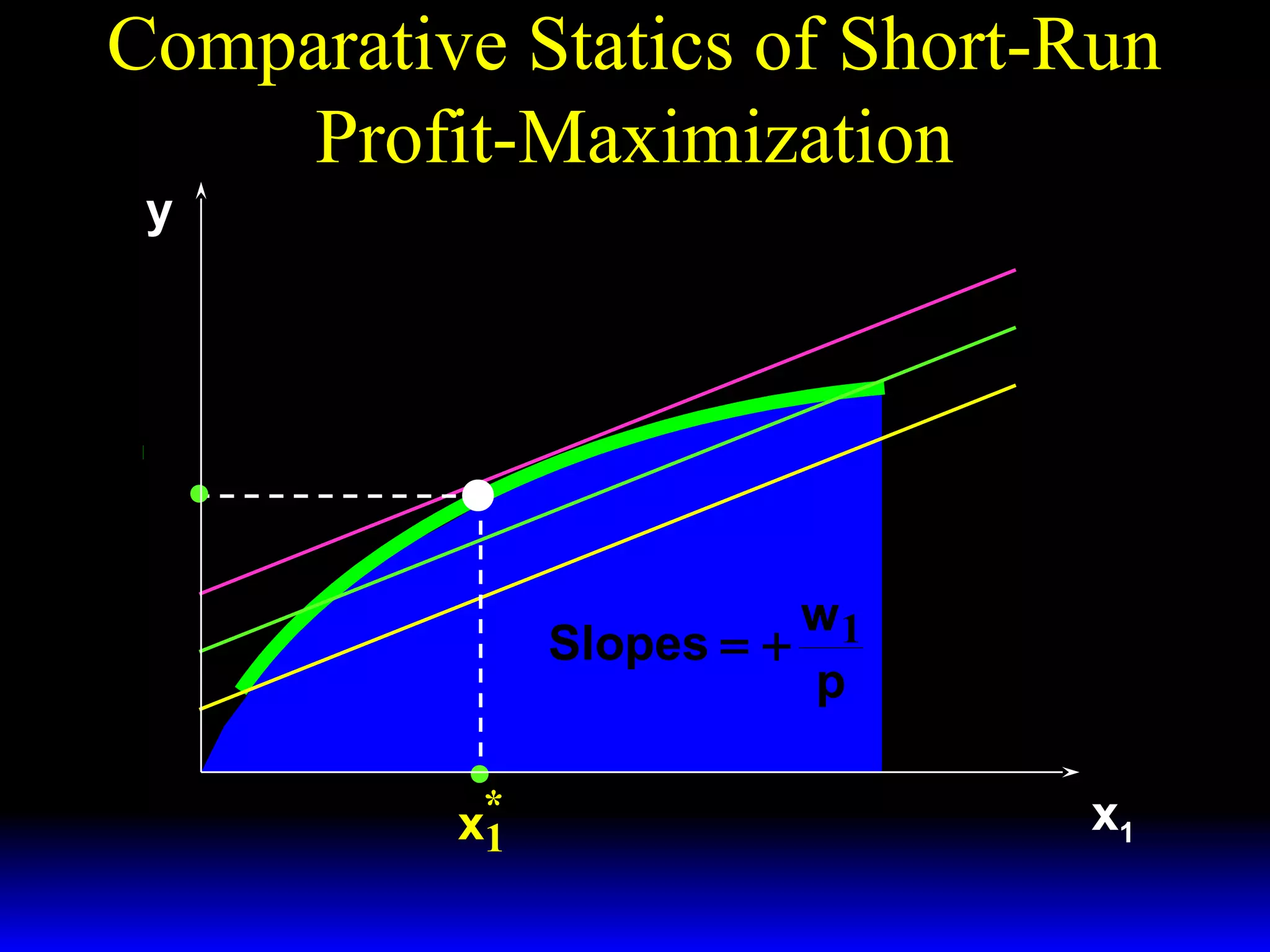
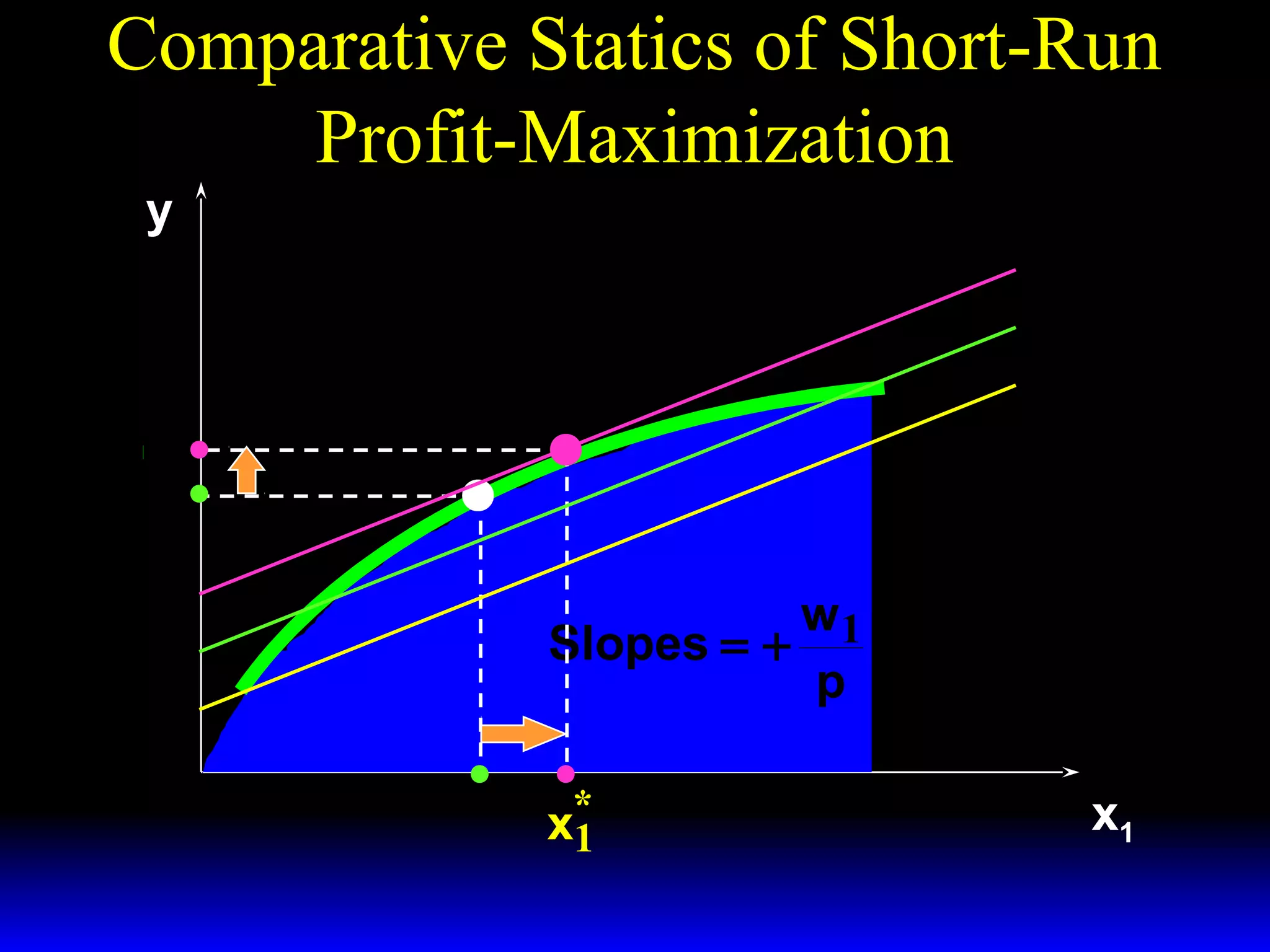
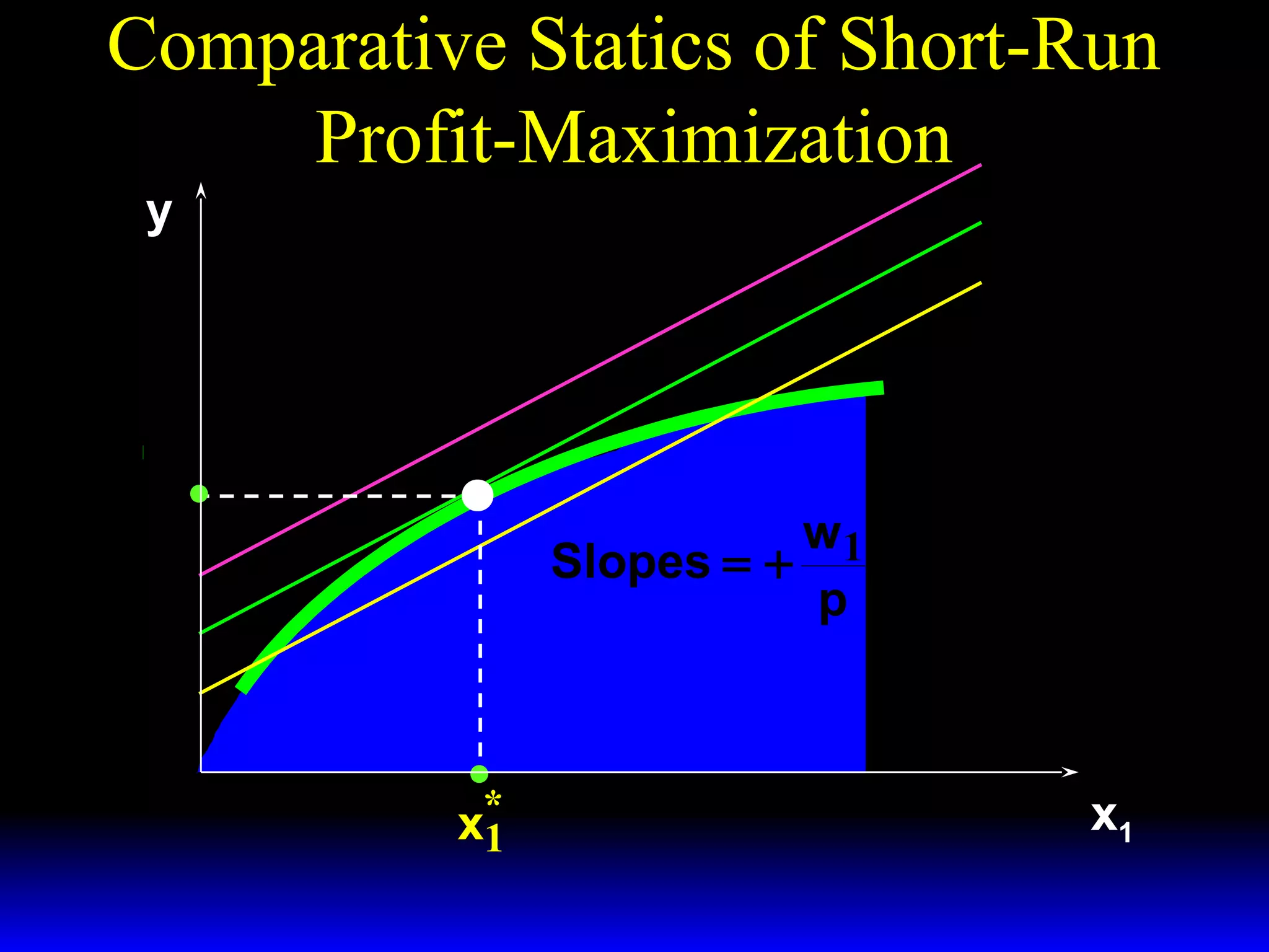
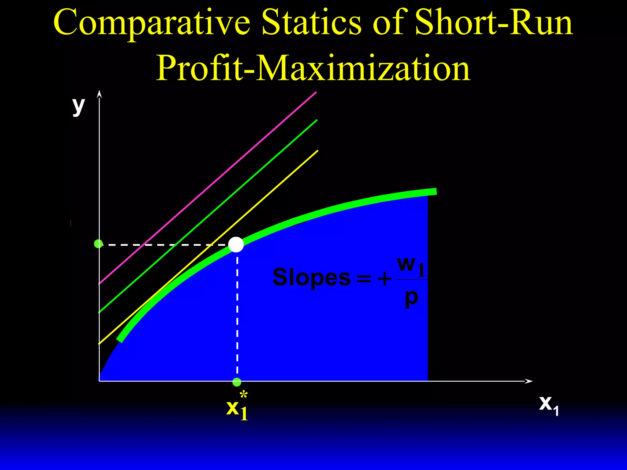
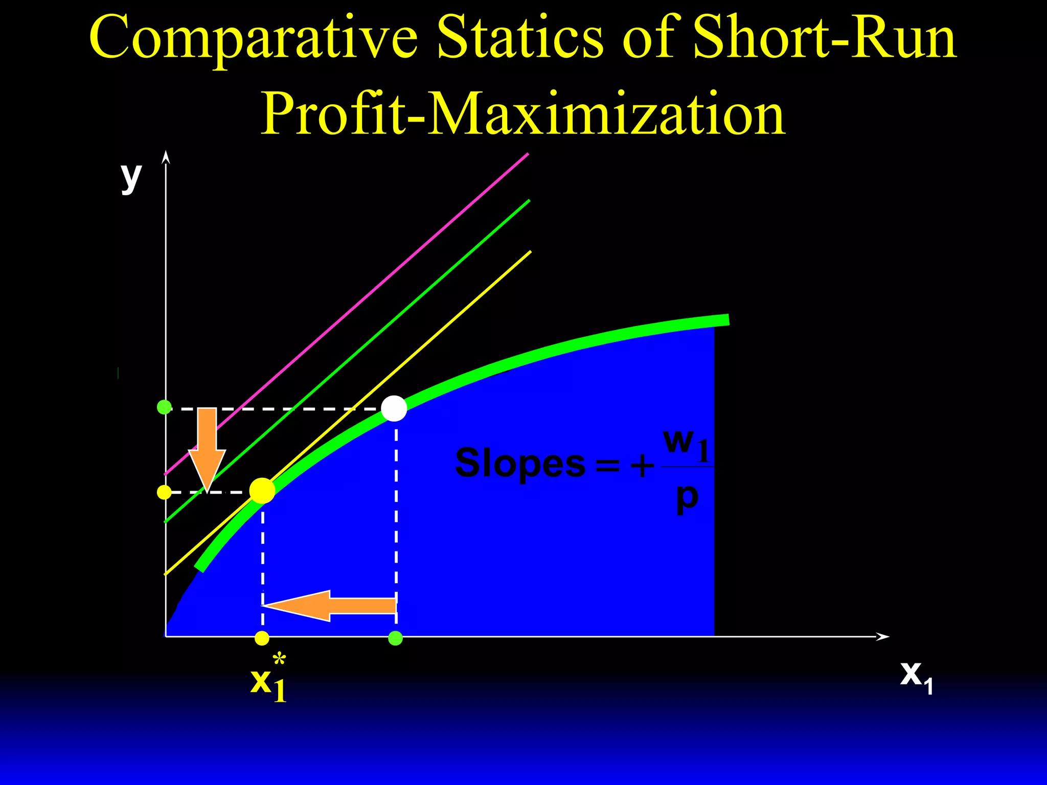
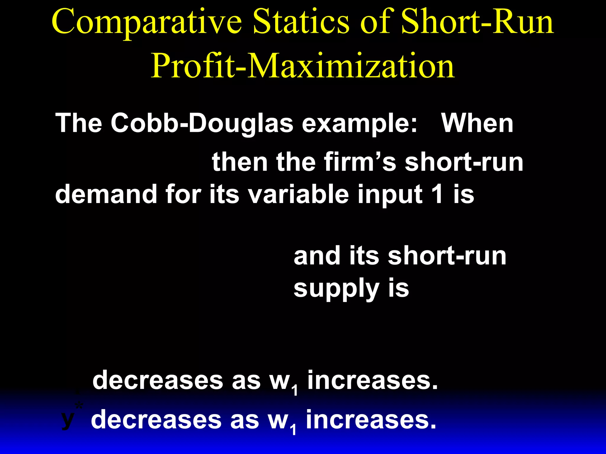
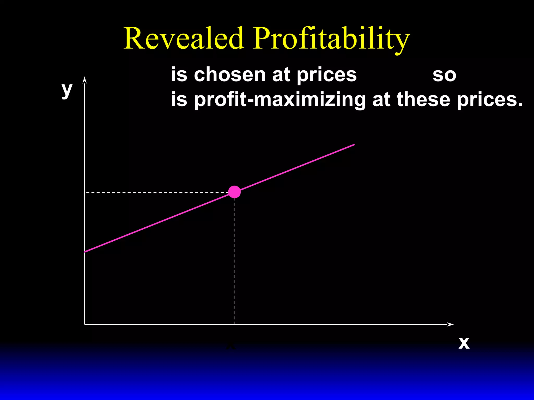
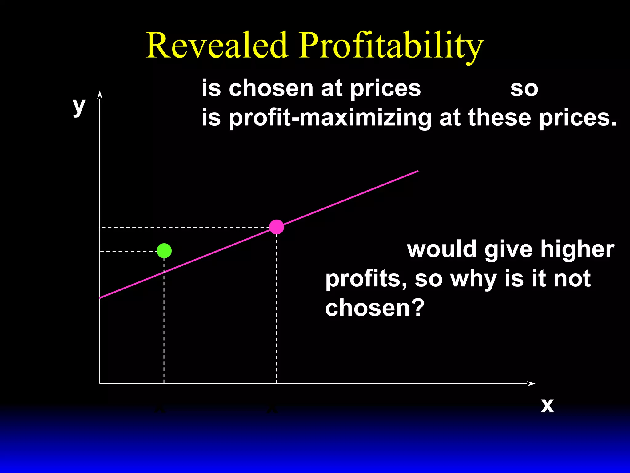
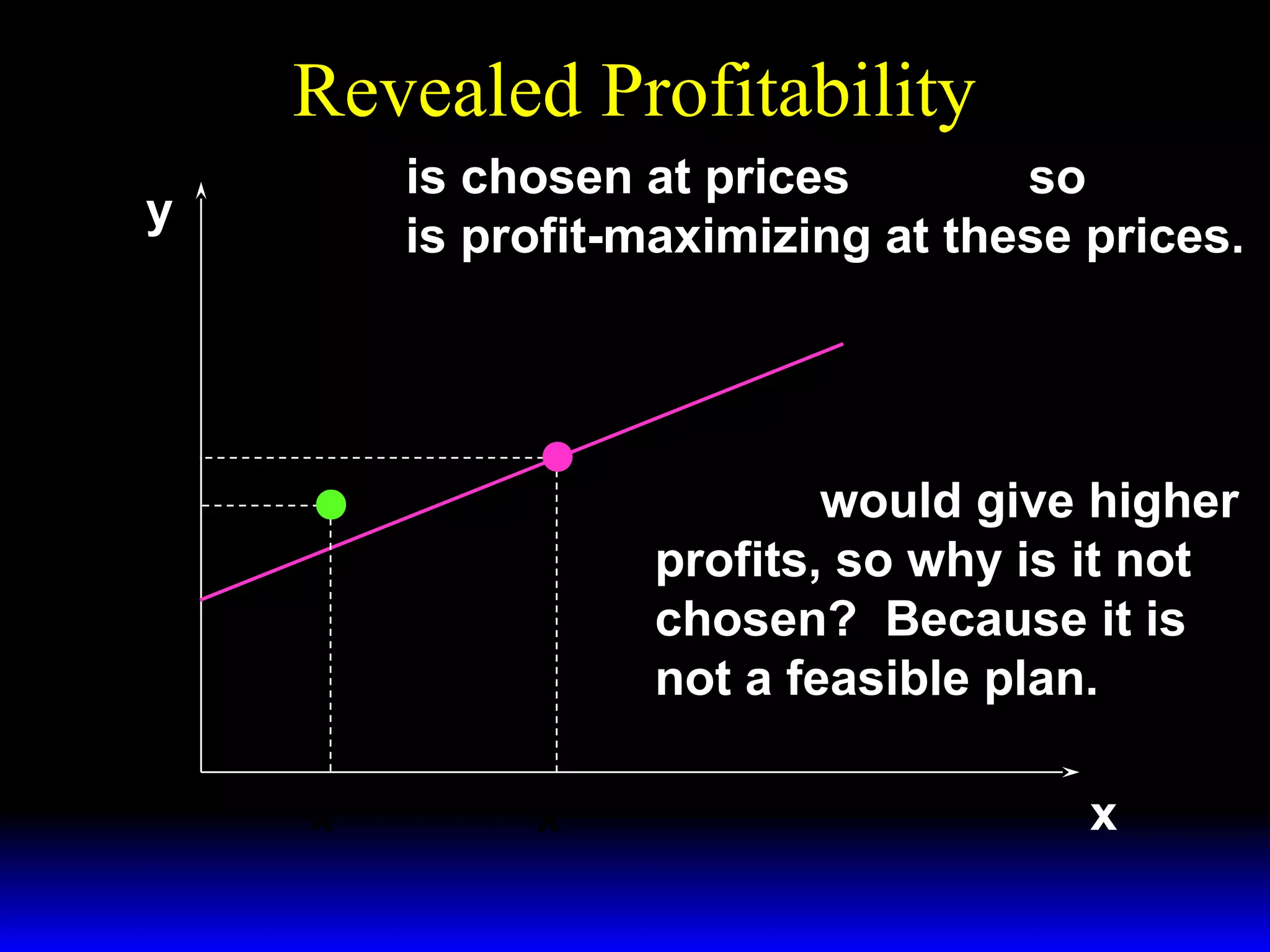
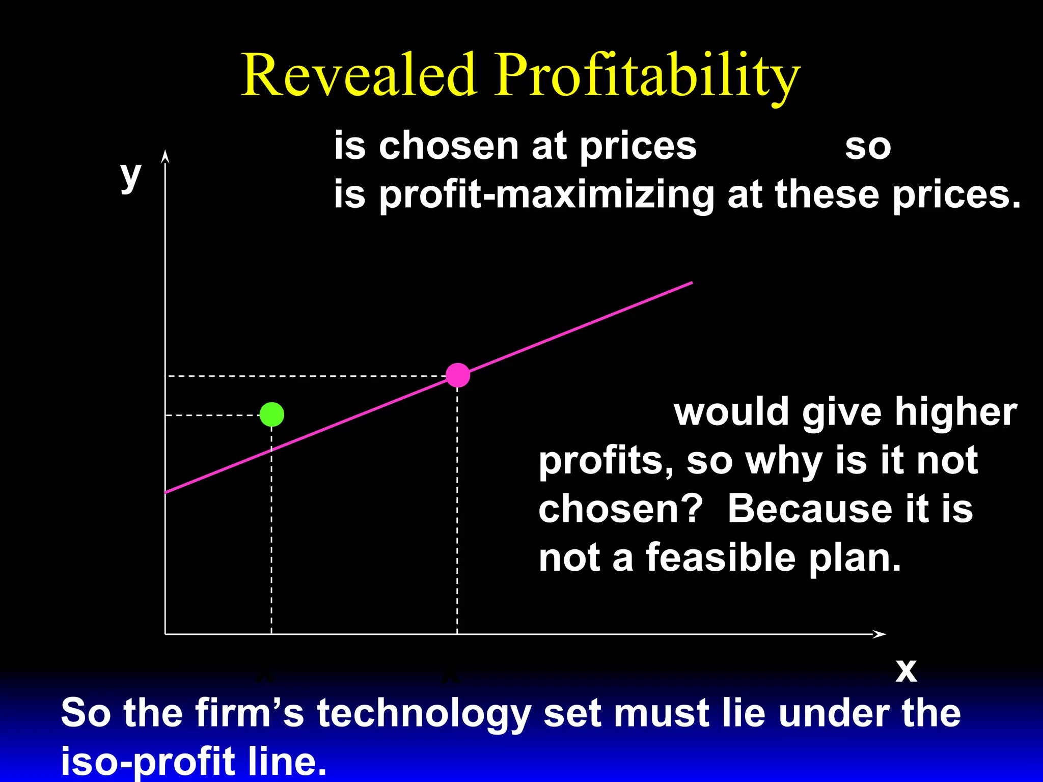
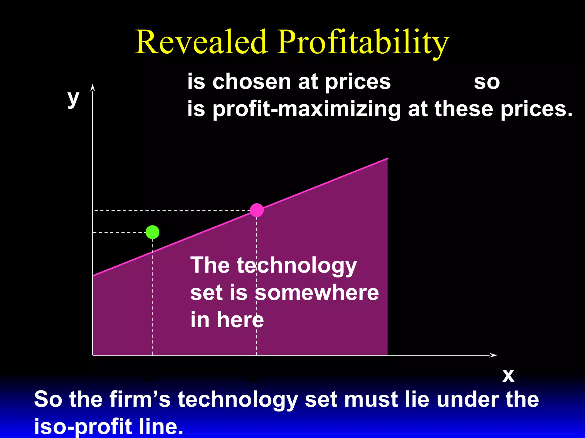
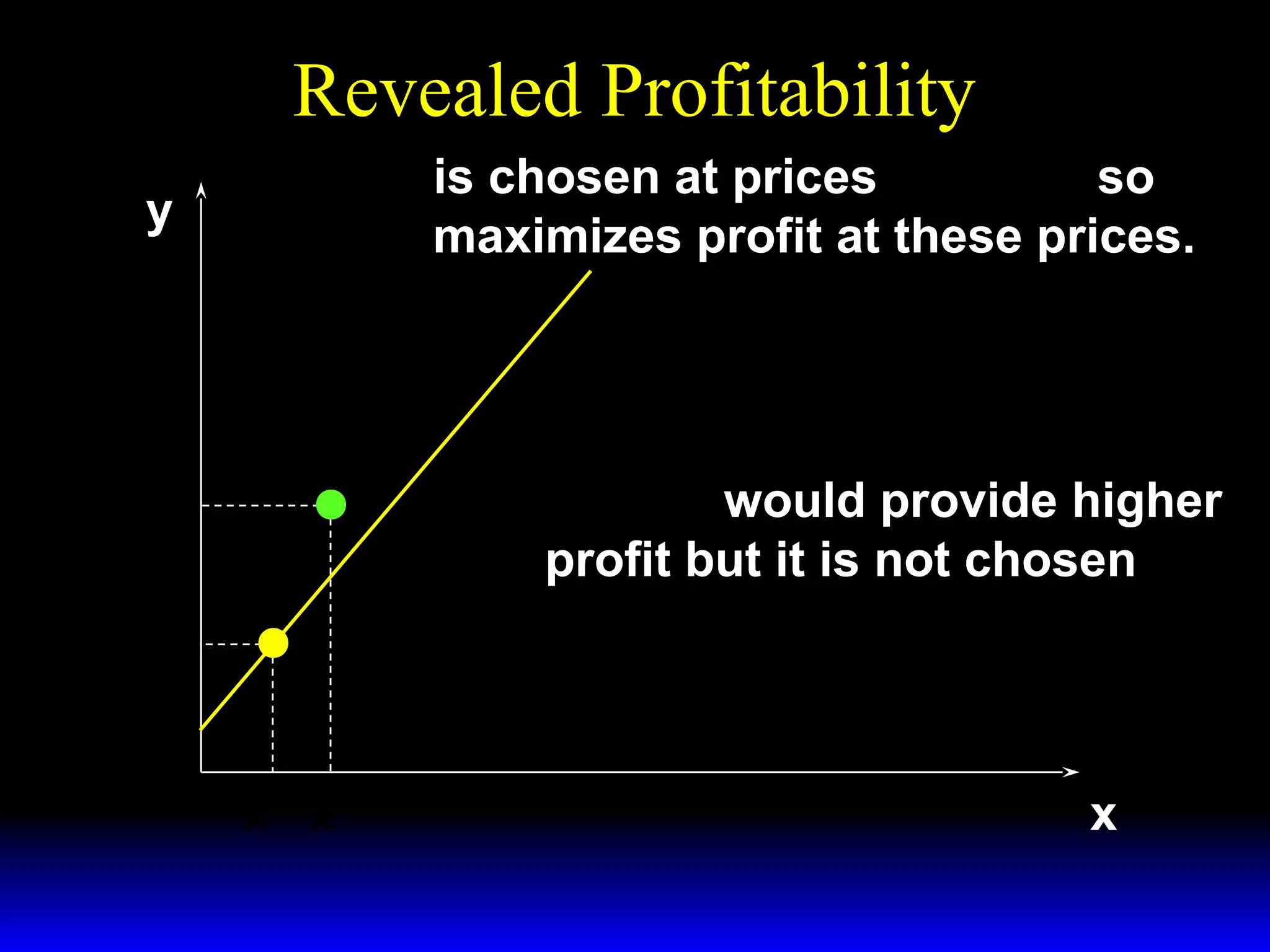
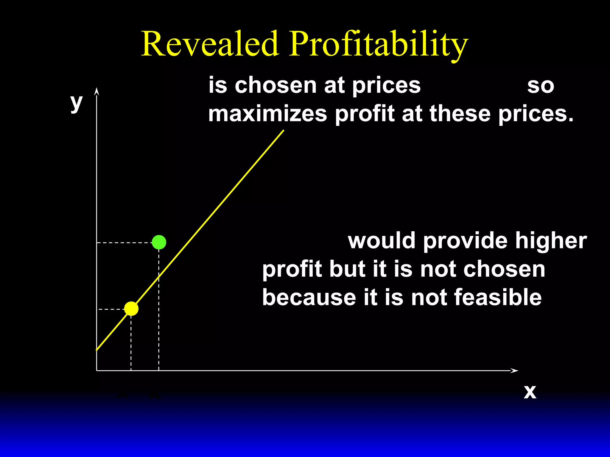
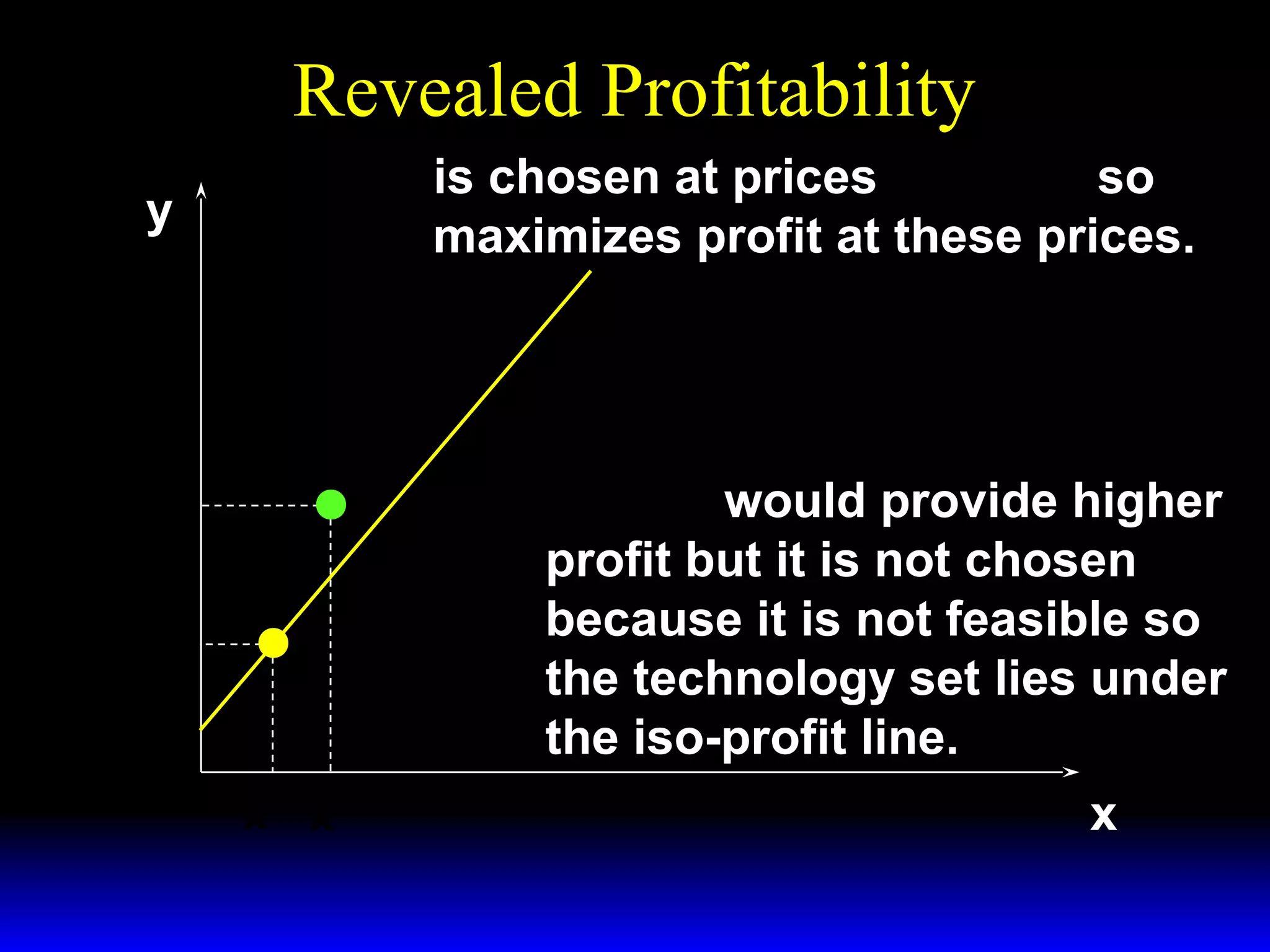
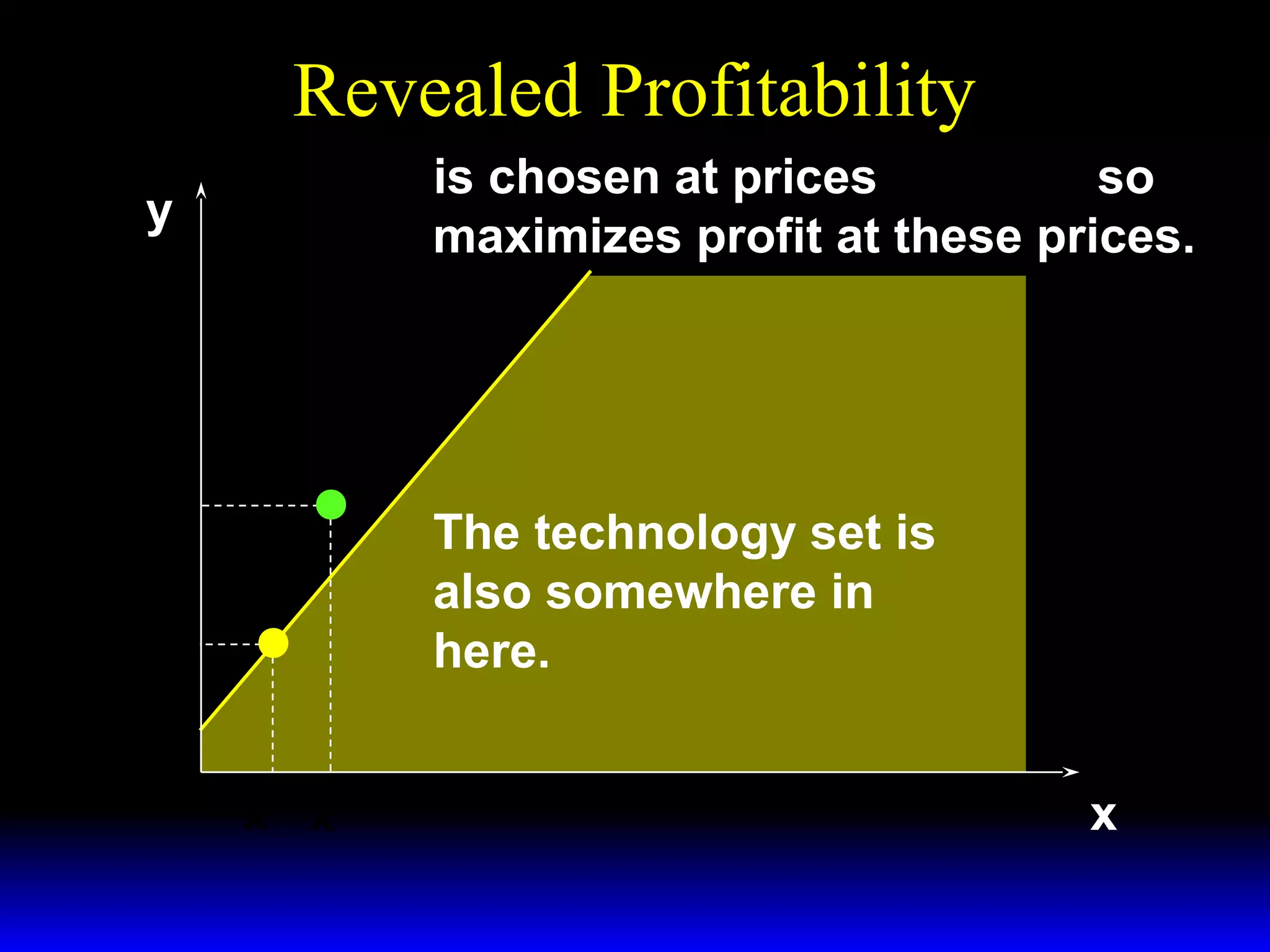
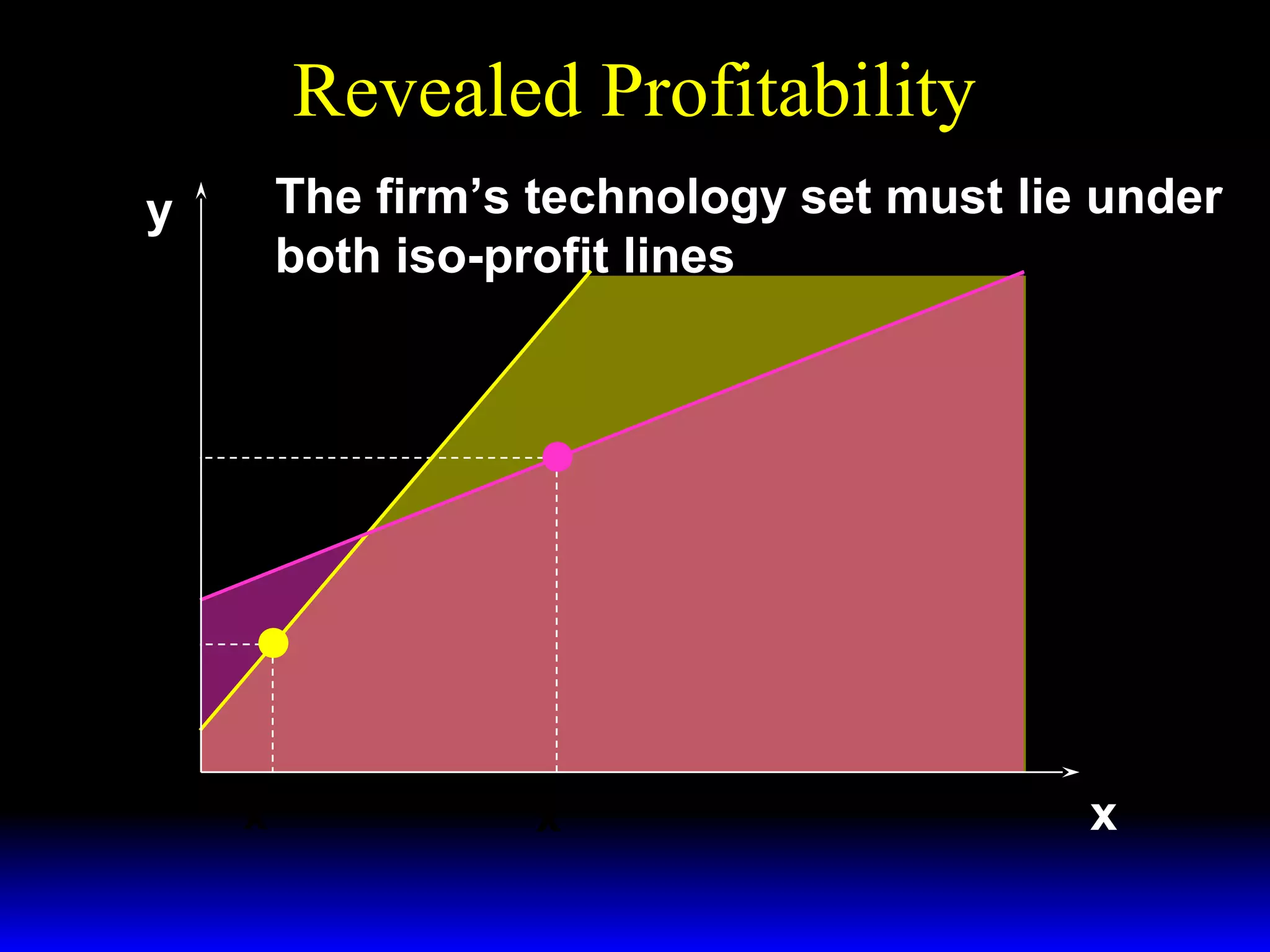
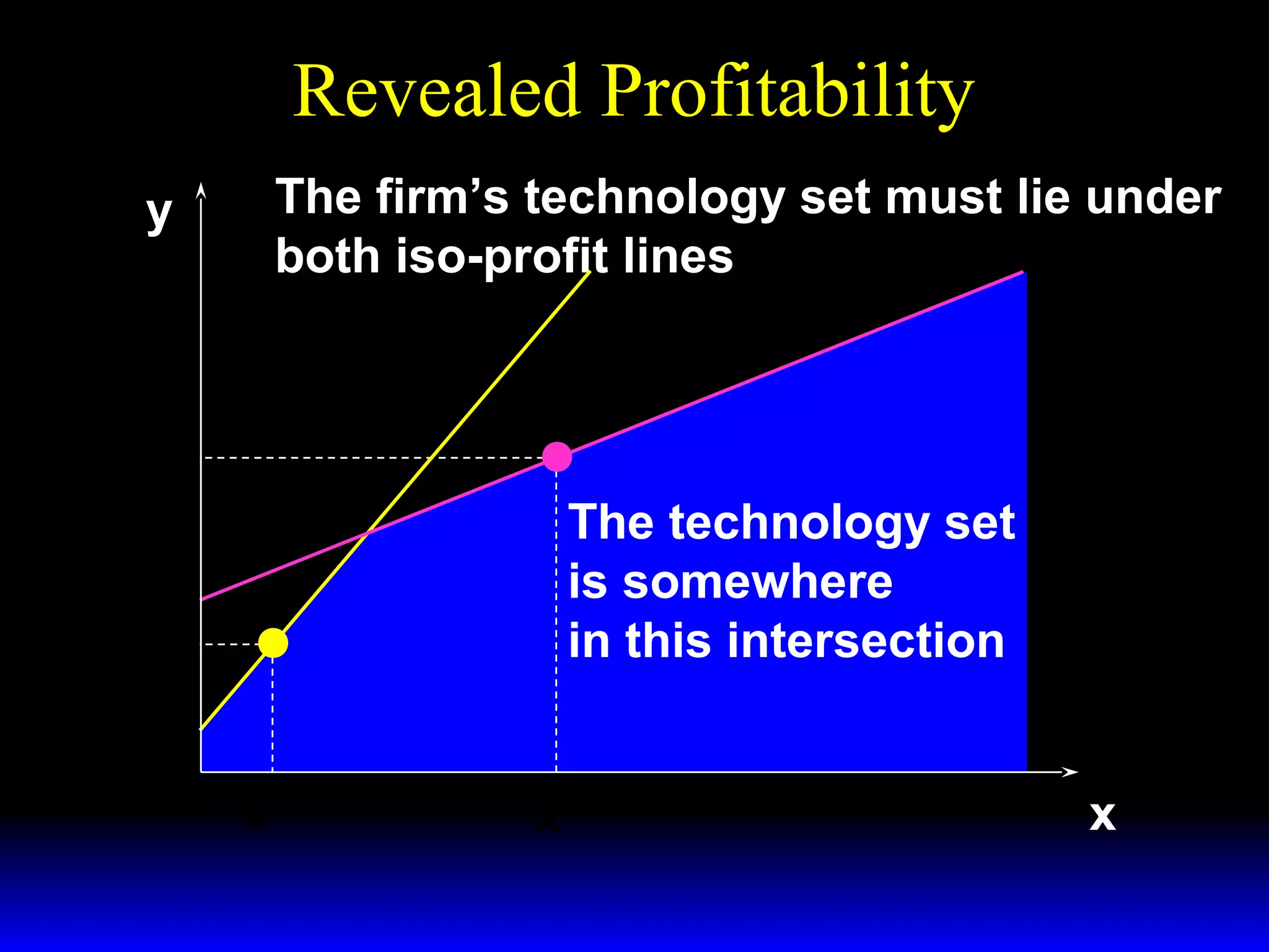
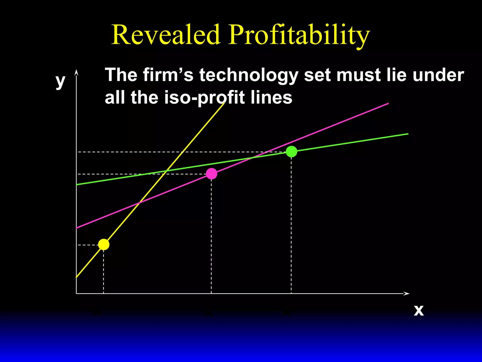
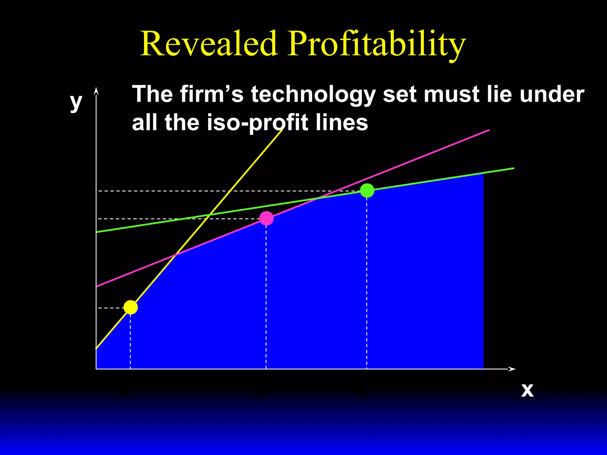
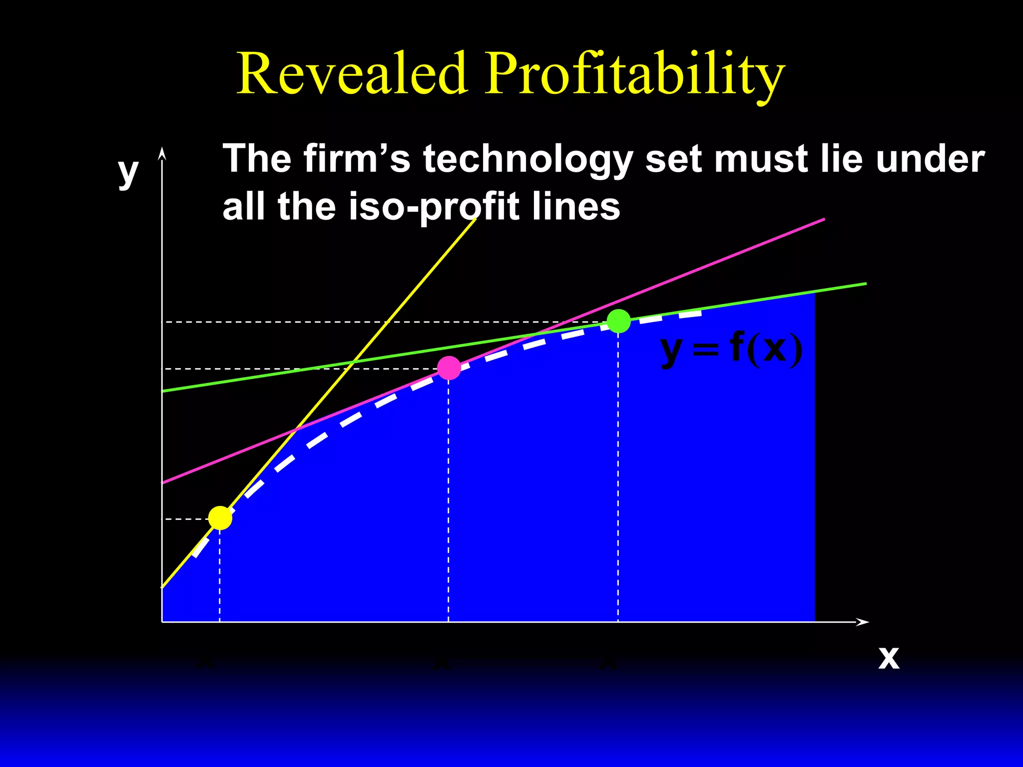
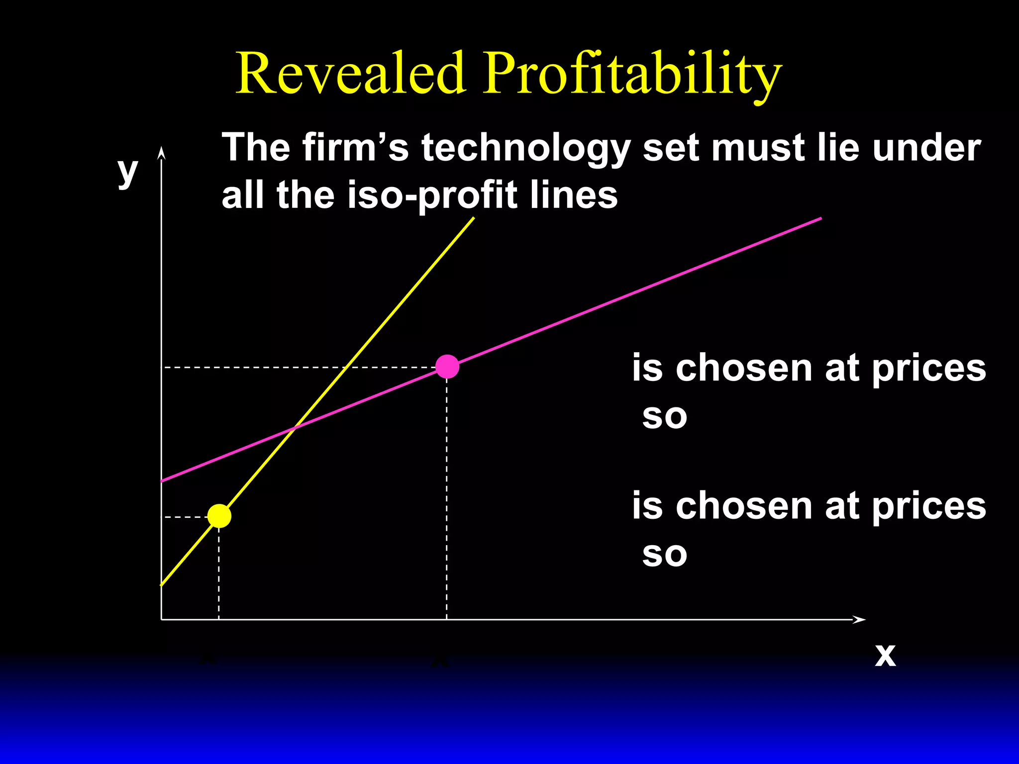
SlideShare a Scribd company logo
1 of 105
Chapter Nineteen
Profit-Maximization
Economic Profit
A firm uses inputs j = 1…,m to make
products i = 1,…n.
Output levels are y1,…,yn.
Input levels are x1,…,xm.
Product prices are p1,…,pn.
Input prices are w1,…,wm.
The Competitive Firm
The competitive firm takes all output
prices p1,…,pn and all input prices w1,
…,wm as given constants.
Economic Profit
The economic profit generated by
the production plan (x1,…,xm,y1,…,yn)
is
Π = p1y1 ++pnyn=− w 1x1 − w mxm .
Π
Economic Profit
Output and input levels are typically
flows.
E.g. x1 might be the number of labor
units used per hour.
And y3 might be the number of cars
produced per hour.
Consequently, profit is typically a
flow also; e.g. the number of dollars
of profit earned per hour.
Economic Profit
How do we value a firm?
Suppose the firm’s stream of
periodic economic profits is
Π 0 , Π 1 , Π 2 , … and r is the rate of
interest.
Then the present-value of the firm’s
economicΠ + Π1 + Πis + 
profit stream 2
PV =
0

1+r

(1 + r ) 2
Economic Profit
A competitive firm seeks to maximize
its present-value.
How?
Economic Profit
Suppose the firm is in a short-run
~ .
circumstance in which x 2 ≡ x 2
Its short-run production function is

~ ).
y = f ( x1 , x 2
Economic Profit
Suppose the firm is in a short-run
~ .
circumstance in which x 2 ≡ x 2
Its short-run production function is

~ ).
y = f ( x1 , x 2

~
The firm’s fixed cost is FC = w 2x 2
and its profit function is
~ .
Π = py − w 1x1 − w 2x 2
Short-Run Iso-Profit Lines
A $Π iso-profit line contains all the
production plans that provide a profit
level $Π .
A $Π iso-profit line’s equation is
~ .
Π ≡ py − w 1x1 − w 2x 2
Short-Run Iso-Profit Lines
A $Π iso-profit line contains all the
production plans that yield a profit
level of $Π .
The equation of a $Π iso-profit line is
~ .
Π ≡ py − w 1x1 − w 2x 2
I.e.
~
w1
Π + w 2x 2
y=
x1 +
.

p

p
Short-Run Iso-Profit Lines
~
w1
Π + w 2x 2
y=
x1 +
p
p

has a slope of

w1
+
p

and a vertical intercept of

~
Π + w 2x 2
.
p
Short-Run Iso-Profit Lines
y

ing
s
ea t
r
nc rofi
I
p

Π ≡ Π′′′
Π ≡ Π′′

Π ≡ Π′

w1
Slopes = +
p

x1
Short-Run Profit-Maximization
The firm’s problem is to locate the
production plan that attains the
highest possible iso-profit line, given
the firm’s constraint on choices of
production plans.
Q: What is this constraint?
Short-Run Profit-Maximization
The firm’s problem is to locate the
production plan that attains the
highest possible iso-profit line, given
the firm’s constraint on choices of
production plans.
Q: What is this constraint?
A: The production function.
Short-Run Profit-Maximization
y

The short-run production function and
~
x2 ≡ x2 .
technology set for

~
y = f ( x1 , x 2 )

Technically
inefficient
plans
x1
Short-Run Profit-Maximization
y

ing
s
ea t
r
nc rofi
I
p

Π ≡ Π′′′
Π ≡ Π′′

Π ≡ Π′

~
y = f ( x1 , x 2 )

w1
Slopes = +
p

x1
Short-Run Profit-Maximization
y

Π ≡ Π′′′
Π ≡ Π′′

Π ≡ Π′

w1
Slopes = +
p

y*

*
x1

x1
Short-Run Profit-Maximization
y

~
Given p, w1 and x 2 ≡ x 2 , the short-run
* ~
*
profit-maximizing plan is ( x1 , x 2 , y ).
Π ≡ Π′′

w1
Slopes = +
p

y*

*
x1

x1
Short-Run Profit-Maximization
y

y*

~
Given p, w1 and x 2 ≡ x 2 , the short-run
* ~
*
profit-maximizing plan is ( x1 , x 2 , y ).
And the maximum
Π ≡ Π′′
possible profit
is Π′′ .
w1
Slopes = +
p

*
x1

x1
Short-Run Profit-Maximization
At the short-run profit-maximizing plan,
y the slopes of the short-run production
function and the maximal Π ≡ Π′′
iso-profit line are
equal.
w1
Slopes = +
y*
p

*
x1

x1
Short-Run Profit-Maximization
At the short-run profit-maximizing plan,
y the slopes of the short-run production
function and the maximal Π ≡ Π′′
iso-profit line are
equal.
w1
Slopes = +
y*
p
w1
MP1 =
p
~
at ( x* , x , y* )
1

*
x1

2

x1
Short-Run Profit-Maximization
w1
MP1 =
p

⇔ p × MP1 = w 1

p × MP1 is the marginal revenue product of

input 1, the rate at which revenue increases
with the amount used of input 1.
If p × MP1 > w1 then profit increases with x 1.
If p × MP1 < w1 then profit decreases with x 1.
Short-Run Profit-Maximization; A
Cobb-Douglas Example
Suppose the short-run production
~
function is y = x1/ 3x1/3 .
1
2
The marginal product of the variable
∂ y 1 − 2/ 3~ 1/ 3
input 1 is
MP1 =
= x1 x 2 .
∂ x1 3
The profit-maximizing condition is
p * − 2/ 3 ~ 1/ 3
MRP1 = p × MP1 = ( x1 )
x2 = w1 .
3
Short-Run Profit-Maximization; A
Cobb-Douglas Example
p * − 2/ 3 ~ 1/ 3
x 2 = w 1 for x1 gives
Solving ( x1 )
3
3w 1
* − 2/ 3
( x1 )
=
.
~
px1/ 3
2
Short-Run Profit-Maximization; A
Cobb-Douglas Example
p * − 2/ 3 ~ 1/ 3
x 2 = w 1 for x1 gives
Solving ( x1 )
3
3w 1
* − 2/ 3
( x1 )
=
.
~
px1/ 3
2

That is,

~
px1/ 3
2
( x* ) 2/ 3 =
1
3w 1
Short-Run Profit-Maximization; A
Cobb-Douglas Example
p * − 2/ 3 ~ 1/ 3
x 2 = w 1 for x1 gives
Solving ( x1 )
3
3w 1
* − 2/ 3
( x1 )
=
.
~
px1/ 3
2

That is,

so

~
px1/ 3
2
( x* ) 2/ 3 =
1
3w 1

~ 1/ 3  3/ 2  p  3/ 2
*  px 2 
~ 1/ 2 .

x1 = 
=
x2


 3w 1 
 3w 1 
Short-Run Profit-Maximization; A
Cobb-Douglas Example
*  p 
x1 = 

 3w 1 

3/ 2

~ 1/ 2
x2

is the firm’s
short-run demand
for input 1 when the level of input 2 is
~
fixed at x 2 units.
Short-Run Profit-Maximization; A
Cobb-Douglas Example
*  p 
x1 = 

 3w 1 

3/ 2

~ 1/ 2
x2

is the firm’s
short-run demand
for input 1 when the level of input 2 is
~
fixed at x 2 units.
The firm’s short-run output level is thus
* 1/ 3 ~ 1/ 3  p 
y = ( x1 ) x 2 = 

 3w 1 
*

1/ 2

~ 1/2 .
x2
Comparative Statics of Short-Run
Profit-Maximization
What happens to the short-run profitmaximizing production plan as the
output price p changes?
Comparative Statics of Short-Run
Profit-Maximization
The equation of a short-run iso-profit line
~
is
w1
Π + w 2x 2
y=
x1 +

p

p

so an increase in p causes
-- a reduction in the slope, and
-- a reduction in the vertical intercept.
Comparative Statics of Short-Run
Profit-Maximization Π ≡ Π′′′
y

Π ≡ Π′′
Π ≡ Π′

~
y = f ( x1 , x 2 )
y*

w1
Slopes = +
p

*
x1

x1
Comparative Statics of Short-Run
Profit-Maximization
y

~
y = f ( x1 , x 2 )
y*

w1
Slopes = +
p
*
x1

x1
Comparative Statics of Short-Run
Profit-Maximization
y

~
y = f ( x1 , x 2 )

y*

w1
Slopes = +
p
*
x1

x1
Comparative Statics of Short-Run
Profit-Maximization
An increase in p, the price of the
firm’s output, causes
– an increase in the firm’s output
level (the firm’s supply curve
slopes upward), and
– an increase in the level of the
firm’s variable input (the firm’s
demand curve for its variable input
shifts outward).
Comparative Statics of Short-Run
Profit-Maximization
The Cobb-Douglas example: When
1/ 3 ~ 1/ 3
y = x1 x 2
then the firm’s short-run
demand for its variable input 1 is
*  p 
x1 = 

 3w 1 

 p 
y =

 3w 1 
*

3/ 2

~ 1/ 2
x2

1/ 2

~
x1/ 2 .
2

and its short-run
supply is
Comparative Statics of Short-Run
Profit-Maximization
The Cobb-Douglas example: When
1/ 3 ~ 1/ 3
y = x1 x 2
then the firm’s short-run
demand for its variable input 1 is
*  p 
x1 = 

 3w 1 

 p 
y =

 3w 1 
*

3/ 2

~ 1/ 2
x2

1/ 2

~
x1/ 2 .
2

and its short-run
supply is

x* increases as p increases.
1
*
y increases as p increases.
Comparative Statics of Short-Run
Profit-Maximization
What happens to the short-run profitmaximizing production plan as the
variable input price w1 changes?
Comparative Statics of Short-Run
Profit-Maximization
The equation of a short-run iso-profit line
~
is
w1
Π + w 2x 2
y=
x1 +

p

p

so an increase in w1 causes
-- an increase in the slope, and
-- no change to the vertical intercept.
Comparative Statics of Short-Run
Profit-Maximization Π ≡ Π′′′
y

Π ≡ Π′′
Π ≡ Π′

~
y = f ( x1 , x 2 )
y*

w1
Slopes = +
p

*
x1

x1
Comparative Statics of Short-Run
Profit-Maximization
Π ≡ Π′′′
Π ≡ Π′′

y

Π ≡ Π′

~
y = f ( x1 , x 2 )
y*

w1
Slopes = +
p

*
x1

x1
Comparative Statics of Short-Run
Profit-Maximization
Π ≡ Π′′′
Π ≡ Π′′

y

Π ≡ Π′

~
y = f ( x1 , x 2 )
w1
Slopes = +
p

y*

*
x1

x1
Comparative Statics of Short-Run
Profit-Maximization
An increase in w1, the price of the
firm’s variable input, causes
– a decrease in the firm’s output
level (the firm’s supply curve shifts
inward), and
– a decrease in the level of the firm’s
variable input (the firm’s demand
curve for its variable input slopes
downward).
Comparative Statics of Short-Run
Profit-Maximization
The Cobb-Douglas example: When
1/ 3 ~ 1/ 3
y = x1 x 2
then the firm’s short-run
demand for its variable input 1 is
*  p 
x1 = 

 3w 1 

 p 
y =

 3w 1 
*

3/ 2

~ 1/ 2
x2
and its short-run

1/ 2

~
x1/ 2 .
2

supply is
Comparative Statics of Short-Run
Profit-Maximization
The Cobb-Douglas example: When
1/ 3 ~ 1/ 3
y = x1 x 2
then the firm’s short-run
demand for its variable input 1 is
*  p 
x1 = 

 3w 1 

 p 
y =

 3w 1 
*

3/ 2

~ 1/ 2
x2
and its short-run

1/ 2

~
x1/ 2 .
2

supply is

x* decreases as w1 increases.
1
y* decreases as w1 increases.
Long-Run Profit-Maximization
Now allow the firm to vary both input
levels.
Since no input level is fixed, there
are no fixed costs.
Long-Run Profit-Maximization
Both x1 and x2 are variable.
Think of the firm as choosing the
production plan that maximizes
profits for a given value of x2, and
then varying x2 to find the largest
possible profit level.
Long-Run Profit-Maximization
The equation of a long-run iso-profit line
is
w1
Π + w 2x 2
y=
x1 +

p

p

so an increase in x2 causes
-- no change to the slope, and
-- an increase in the vertical intercept.
Long-Run Profit-Maximization
y

y = f ( x1 , x ′ )
2

x1
Long-Run Profit-Maximization
y
y = f ( x1 , 3x ′ )
2
y = f ( x1 , 2x′ )
2

y = f ( x1 , x ′ )
2

Larger levels of input 2 increase the
productivity of input 1.

x1
Long-Run Profit-Maximization
y
y = f ( x1 , 3x ′ )
2
y = f ( x1 , 2x′ )
2

y = f ( x1 , x ′ )
2

The marginal product
of input 2 is
diminishing.
Larger levels of input 2 increase the
productivity of input 1.

x1
Long-Run Profit-Maximization
y
y = f ( x1 , 3x ′ )
2
y = f ( x1 , 2x′ )
2

y = f ( x1 , x ′ )
2

The marginal product
of input 2 is
diminishing.
Larger levels of input 2 increase the
productivity of input 1.

x1
Long-Run Profit-Maximization
y

p × MP1 − w 1 = 0 for each short-run

production plan.

y = f ( x1 , 3x ′ )
2
y = f ( x1 , 2x′ )
2

y* ( 3x ′ )
2
y* ( 2x ′ )
2

y = f ( x1 , x ′ )
2

*

y ( x′ )
2
x* ( x ′ )
x* ( 3x′ )
1 2
1
2
*
x1 ( 2x′ )
2

x1
Long-Run Profit-Maximization
y

p × MP1 − w 1 = 0 for each short-run

production plan.

y = f ( x1 , 3x ′ )
2
y = f ( x1 , 2x′ )
2

y* ( 3x ′ )
2
y* ( 2x ′ )
2

y = f ( x1 , x ′ )
2

The marginal product
of input 2 is
diminishing so ...

*

y ( x′ )
2
x* ( x ′ )
x* ( 3x′ )
1 2
1
2
*
x1 ( 2x′ )
2

x1
Long-Run Profit-Maximization
y

p × MP1 − w 1 = 0 for each short-run

production plan.

y = f ( x1 , 3x ′ )
2
y = f ( x1 , 2x′ )
2

y* ( 3x ′ )
2
y* ( 2x ′ )
2

y = f ( x1 , x ′ )
2

the marginal profit
of input 2 is
diminishing.

*

y ( x′ )
2
x* ( x ′ )
x* ( 3x′ )
1 2
1
2
*
x1 ( 2x′ )
2

x1
Long-Run Profit-Maximization
Profit will increase as x2 increases so
long as the marginal profit of input 2
p × MP2 − w 2 > 0.

The profit-maximizing level of input 2
therefore satisfies
p × MP2 − w 2 = 0.
Long-Run Profit-Maximization
Profit will increase as x2 increases so
long as the marginal profit of input 2
p × MP2 − w 2 > 0.

The profit-maximizing level of input 2
therefore satisfies
p × MP2 − w 2 = 0.

And p × MP1 − w1 = 0 is satisfied in
any short-run, so ...
Long-Run Profit-Maximization
The input levels of the long-run
profit-maximizing plan satisfy
p × MP1 − w 1 = 0 and p × MP2 − w 2 = 0.

That is, marginal revenue equals
marginal cost for all inputs.
Long-Run Profit-Maximization
The Cobb-Douglas example: When
1/ 3 ~ 1/ 3
y = x1 x 2 then the firm’s short-run
demand for its variable input 1 is
*  p 
x1 = 

 3w 1 

 p 
y =

 3w 1 
*

3/ 2

~ 1/ 2
x2

1/ 2

~
x1/ 2 .
2

and its short-run
supply is

Short-run profit is therefore …
Long-Run Profit-Maximization
~
Π = py* − w 1x* − w 2x 2
1
 p 
= p

 3w 1 

1/ 2

~ 1/ 2 − w  p 
x2

1
 3w 1 

3/ 2

~
~
x1/ 2 − w 2x 2
2
Long-Run Profit-Maximization
~
Π = py* − w 1x* − w 2x 2
1
 p 
= p

 3w 1 

1/ 2

 p 
= p

 3w 1 

1/ 2

~ 1/ 2 − w  p 
x2

1
 3w 1 

3/ 2

~
~
x1/ 2 − w 2x 2
2

~ 1/ 2 − w p  p 
x2


1
3w 1  3w 1 

1/ 2

~
− w 2x 2
Long-Run Profit-Maximization
~
Π = py* − w 1x* − w 2x 2
1
 p 
= p

 3w 1 

1/ 2

 p 
= p

 3w 1 

1/ 2

2p  p 
=


3  3w 1 

~ 1/ 2 − w  p 
x2

1
 3w 1 

3/ 2

~
~
x1/ 2 − w 2x 2
2

~ 1/ 2 − w p  p 
x2


1
3w 1  3w 1 

1/ 2

~
~
x1/ 2 − w 2x 2
2

1/ 2

~
− w 2x 2
Long-Run Profit-Maximization
~
Π = py* − w 1x* − w 2x 2
1
 p 
= p

 3w 1 

1/ 2

 p 
= p

 3w 1 

1/ 2

2p  p 
=


3  3w 1 

~ 1/ 2 − w  p 
x2

1
 3w 1 

3/ 2

~
~
x1/ 2 − w 2x 2
2

~ 1/ 2 − w p  p 
x2


1
3w 1  3w 1 

1/ 2

~
~
x1/ 2 − w 2x 2
2

3  1/ 2
 4p
~
~

=
x1/ 2 − w 2x 2 .
2
 27w 

1

1/ 2

~
− w 2x 2
Long-Run Profit-Maximization
3  1/ 2
 4p
~
~

Π=
x1/ 2 − w 2x 2 .
2
 27w 

1

What is the long-run profit-maximizing
level of input 2? Solve
3  1/ 2
∂ Π 1  4p
~−

0= ~ = 
x 2 1/ 2 − w 2
∂ x 2 2  27w 1 



to get

~
x 2 = x* =
2

p3
27w 1w 2
2

.
Long-Run Profit-Maximization
What is the long-run profit-maximizing
input 1 level? Substitute
x* =
2

p

3

27w 1w 2
2

to get

into

*  p 
x1 = 

 3w 1 

3/ 2

~
x1/ 2
2
Long-Run Profit-Maximization
What is the long-run profit-maximizing
input 1 level? Substitute
x* =
2

p

3

into

27w 1w 2
2

*  p 
x1 = 

 3w 1 

3/ 2

~
x1/ 2
2

to get
*  p 
x1 = 

 3w 1 

3 / 2


p



2
 27w 1w 2 
3

1/ 2

=

p

3

2
27w 1 w 2

.
Long-Run Profit-Maximization
What is the long-run profit-maximizing
output level? Substitute
x* =
2

p

3

27w 1w 2
2

to get

 p 
into y = 

 3w 1 
*

1/ 2

~
x1/ 2
2
Long-Run Profit-Maximization
What is the long-run profit-maximizing
output level? Substitute
x* =
2

p

 p 
into y = 

 3w 1 

3

*

27w 1w 2
2

1/ 2

~
x1/ 2
2

to get
*  p 
y =

 3w 1 

1/ 2





2
 27w 1w 2 
p

3

1/ 2

p2
=
.
9 w 1w 2
Long-Run Profit-Maximization
So given the prices p, w 1 and w2, and
the production function y = x1/ 3x1/ 3
1
2
the long-run profit-maximizing production
plan is

p3
p3
p2 
.
( x* , x* , y* ) = 
,
,
1 2


2
 27w 1 w 2 27w 1w 2 9 w 1w 2 
2
Returns-to-Scale and ProfitMaximization
If a competitive firm’s technology
exhibits decreasing returns-to-scale
then the firm has a single long-run
profit-maximizing production plan.
Returns-to Scale and ProfitMaximization
y

y = f(x)
y*

Decreasing
returns-to-scale
x*

x
Returns-to-Scale and ProfitMaximization
If a competitive firm’s technology
exhibits exhibits increasing returnsto-scale then the firm does not have
a profit-maximizing plan.
Returns-to Scale and ProfitMaximization
y
g
asin
ncre it
I
prof

y = f(x)

y”
y’

Increasing
returns-to-scale
x’

x”

x
Returns-to-Scale and ProfitMaximization
So an increasing returns-to-scale
technology is inconsistent with firms
being perfectly competitive.
Returns-to-Scale and ProfitMaximization
What if the competitive firm’s
technology exhibits constant
returns-to-scale?
Returns-to Scale and ProfitMaximization
y
g
asin
ncre it
I
prof

y = f(x)

y”

Constant
returns-to-scale

y’
x’

x”

x
Returns-to Scale and ProfitMaximization
So if any production plan earns a
positive profit, the firm can double
up all inputs to produce twice the
original output and earn twice the
original profit.
Returns-to Scale and ProfitMaximization
Therefore, when a firm’s technology
exhibits constant returns-to-scale,
earning a positive economic profit is
inconsistent with firms being
perfectly competitive.
Hence constant returns-to-scale
requires that competitive firms earn
economic profits of zero.
Returns-to Scale and ProfitMaximization
y

y = f(x)

Π =0
y”

Constant
returns-to-scale

y’
x’

x”

x
Revealed Profitability
Consider a competitive firm with a
technology that exhibits decreasing
returns-to-scale.
For a variety of output and input
prices we observe the firm’s choices
of production plans.
What can we learn from our
observations?
Revealed Profitability
If a production plan (x’,y’) is chosen
at prices (w’,p’) we deduce that the
plan (x’,y’) is revealed to be profitmaximizing for the prices (w’,p’).
Revealed Profitability
y

( x′ , y′ ) is chosen at prices ( w ′ , p′ )

w′
Slope =
p′
y′

x′

x
Revealed Profitability
y

( x′ , y′ ) is chosen at prices ( w ′ , p′ ) so

( x′ , y′ ) is profit-maximizing at these prices.

w′
Slope =
p′
y′

x′

x
Revealed Profitability
y

( x′ , y′ ) is chosen at prices ( w ′ , p′ ) so

( x′ , y′ ) is profit-maximizing at these prices.

w′
Slope =
p′
y′
y′′

( x′′ , y′′ ) would give higher

profits, so why is it not
chosen?

x′′

x′

x
Revealed Profitability
y

( x′ , y′ ) is chosen at prices ( w ′ , p′ ) so

( x′ , y′ ) is profit-maximizing at these prices.

w′
Slope =
p′
y′
y′′

( x′′ , y′′ ) would give higher

profits, so why is it not
chosen? Because it is
not a feasible plan.
x′′

x′

x
Revealed Profitability
y

( x′ , y′ ) is chosen at prices ( w ′ , p′ ) so

( x′ , y′ ) is profit-maximizing at these prices.

w′
Slope =
p′
y′
y′′

( x′′ , y′′ ) would give higher

profits, so why is it not
chosen? Because it is
not a feasible plan.
x
x′
So the firm’s technology set must lie under the
iso-profit line.
x′′
Revealed Profitability
y

( x′ , y′ ) is chosen at prices ( w ′ , p′ ) so

( x′ , y′ ) is profit-maximizing at these prices.

w′
Slope =
p′
y′
y′′

The technology
set is somewhere
in here
x
x′
So the firm’s technology set must lie under the
iso-profit line.
x′′
Revealed Profitability
y

( x′′′ , y′′′ ) is chosen at prices ( w ′′′ , p′′′ ) so
( x′′′ , y′′′ ) maximizes profit at these prices.

w ′′′
Slope =
p′′′
( x ′′ , y′′ ) would provide higher

y′′

profit but it is not chosen
y′′′

x ′′′ x ′′

x
Revealed Profitability
y

( x′′′ , y′′′ ) is chosen at prices ( w ′′′ , p′′′ ) so
( x′′′ , y′′′ ) maximizes profit at these prices.

w ′′′
Slope =
p′′′
y′′

( x ′′ , y′′ ) would provide higher

y′′′

profit but it is not chosen
because it is not feasible

x ′′′ x ′′

x
Revealed Profitability
y

( x′′′ , y′′′ ) is chosen at prices ( w ′′′ , p′′′ ) so
( x′′′ , y′′′ ) maximizes profit at these prices.

w ′′′
Slope =
p′′′
y′′

( x ′′ , y′′ ) would provide higher

y′′′

profit but it is not chosen
because it is not feasible so
the technology set lies under
the iso-profit line.
x ′′′ x ′′

x
Revealed Profitability
y

( x′′′ , y′′′ ) is chosen at prices ( w ′′′ , p′′′ ) so
( x′′′ , y′′′ ) maximizes profit at these prices.

w ′′′
Slope =
p′′′
y′′

The technology set is
also somewhere in
here.

y′′′

x ′′′ x ′′

x
Revealed Profitability
y

The firm’s technology set must lie under
both iso-profit lines

y′

y′′′

x ′′′

x′

x
Revealed Profitability
y

The firm’s technology set must lie under
both iso-profit lines

y′

The technology set
is somewhere
in this intersection

y′′′

x ′′′

x′

x
Revealed Profitability
Observing more choices of
production plans by the firm in
response to different prices for its
input and its output gives more
information on the location of its
technology set.
Revealed Profitability
y

The firm’s technology set must lie under
all the iso-profit lines
( w ′ , p′ )
( w ′′′ , p′′′ )

y′′
y′

( w ′′ , p′′ )

y′′′

x ′′′

x′

x′′

x
Revealed Profitability
y

The firm’s technology set must lie under
all the iso-profit lines
( w ′ , p′ )
( w ′′′ , p′′′ )

y′′
y′

( w ′′ , p′′ )

y′′′

x ′′′

x′

x′′

x
Revealed Profitability
y

The firm’s technology set must lie under
all the iso-profit lines
( w ′ , p′ )
( w ′′′ , p′′′ )

y′′
y′

( w ′′ , p′′ )

y = f(x)

y′′′

x ′′′

x′

x′′

x
Revealed Profitability
What else can be learned from the
firm’s choices of profit-maximizing
production plans?
Revealed Profitability
y

The firm’s technology set must lie under
all the iso-profit lines
( w ′ , p′ )
( w ′′ , p′′ )

( x′ , y′ ) is chosen at prices
( w ′ , p′ ) so

y′

p′ y′ − w ′x ′ ≥ p′ y′′ − w ′x′′ .
( x′′ , y′′ ) is chosen at prices

y′′

( w ′′ , p′′ ) so

p′′ y′′ − w ′′x′′ ≥ p′′ y′ − w ′′x′ .

x ′′

x′

x
Revealed Profitability
p′y′ − w ′x ′ ≥ p′y′′ − w ′x ′′ and

p′′y′′ − w ′′x ′′ ≥ p′′y′ − w ′′x ′ so
p′y′ − w ′x ′ ≥ p′y′′ − w ′x ′′ and

− p′′y′ + w ′′x ′ ≥ − p′′y′′ + w ′′x ′′.

Adding gives
( p′ −p′ ) y′ −( w ′ −w ′ ) x ′ ≥
′
′
( p′ −p′ ) y′ −( w ′ −w ′ ) x ′ .
′
′
′
′
Revealed Profitability
( p′ − p′′ ) y′ − ( w ′ − w ′′ ) x ′ ≥
( p′ − p′′ ) y′′ − ( w ′ − w ′′ ) x ′′
so

( p′ − p′′ )( y′ − y′′ ) ≥ ( w ′ − w ′′ )( x ′ − x ′′ )
That is,

∆p∆y ≥ ∆w∆x

is a necessary implication of profitmaximization.
Revealed Profitability
∆ ∆ ≥∆ ∆
p y
w x

is a necessary implication of profitmaximization.
Suppose the input price does not change.
Then ∆w = 0 and profit-maximization
p y
implies ∆ ∆ ≥0; i.e., a competitive
firm’s output supply curve cannot slope
downward.
Revealed Profitability
∆ ∆ ≥∆ ∆
p y
w x

is a necessary implication of profitmaximization.
Suppose the output price does not change.
Then ∆p = 0 and profit-maximization
w x
implies 0 ≥∆ ∆; i.e., a competitive
firm’s input demand curve cannot slope
upward.

More Related Content

What's hot

Principles of Microeconomics Notes
Principles of Microeconomics NotesPrinciples of Microeconomics Notes
Principles of Microeconomics NotesLaurel Ayuyao
 
History of Economic Thought
History of Economic ThoughtHistory of Economic Thought
History of Economic ThoughtJohn Cousins
 
Chapter 07 presentation
Chapter 07 presentationChapter 07 presentation
Chapter 07 presentationjohn3092
 
Chapter 12 monopolistic and oligopoly
Chapter 12 monopolistic and oligopolyChapter 12 monopolistic and oligopoly
Chapter 12 monopolistic and oligopolyYesica Adicondro
 
Solving Quadratics by Completing the Square
Solving Quadratics by Completing the SquareSolving Quadratics by Completing the Square
Solving Quadratics by Completing the Squareswartzje
 
Perfect competition
Perfect competitionPerfect competition
Perfect competitionAnnie1199
 
Engineering Economics (Cost Function)
Engineering Economics  (Cost Function)Engineering Economics  (Cost Function)
Engineering Economics (Cost Function)GAURAV. H .TANDON
 
Perfect competition
Perfect competitionPerfect competition
Perfect competitiondomsr
 
Disequilibrium Continued
Disequilibrium ContinuedDisequilibrium Continued
Disequilibrium ContinuedSam Georgi
 
Chapter 07 Consumers, Producers And The Efficiency Of Market
Chapter 07   Consumers, Producers And The Efficiency Of MarketChapter 07   Consumers, Producers And The Efficiency Of Market
Chapter 07 Consumers, Producers And The Efficiency Of Marketsira78
 
Straight Lines ( Especially For XI )
Straight Lines ( Especially For XI ) Straight Lines ( Especially For XI )
Straight Lines ( Especially For XI ) Atit Gaonkar
 
Market Equilibrium
Market EquilibriumMarket Equilibrium
Market Equilibriumitutor
 
Distance Between Two Points.pptx
Distance Between Two Points.pptxDistance Between Two Points.pptx
Distance Between Two Points.pptxMartinGeraldine
 
Chapter 4 individual and market demand
Chapter 4 individual and market demandChapter 4 individual and market demand
Chapter 4 individual and market demandYesica Adicondro
 

What's hot (20)

Principles of Microeconomics Notes
Principles of Microeconomics NotesPrinciples of Microeconomics Notes
Principles of Microeconomics Notes
 
History of Economic Thought
History of Economic ThoughtHistory of Economic Thought
History of Economic Thought
 
Chapter 07 presentation
Chapter 07 presentationChapter 07 presentation
Chapter 07 presentation
 
Chapter 12 monopolistic and oligopoly
Chapter 12 monopolistic and oligopolyChapter 12 monopolistic and oligopoly
Chapter 12 monopolistic and oligopoly
 
st petersburg paradox
st petersburg paradoxst petersburg paradox
st petersburg paradox
 
Solving Quadratics by Completing the Square
Solving Quadratics by Completing the SquareSolving Quadratics by Completing the Square
Solving Quadratics by Completing the Square
 
Perfect competition
Perfect competitionPerfect competition
Perfect competition
 
Engineering Economics (Cost Function)
Engineering Economics  (Cost Function)Engineering Economics  (Cost Function)
Engineering Economics (Cost Function)
 
Perfect competition
Perfect competitionPerfect competition
Perfect competition
 
Disequilibrium Continued
Disequilibrium ContinuedDisequilibrium Continued
Disequilibrium Continued
 
Ch12
Ch12Ch12
Ch12
 
Budget lines
Budget linesBudget lines
Budget lines
 
Oligopoly
OligopolyOligopoly
Oligopoly
 
Chapter 07 Consumers, Producers And The Efficiency Of Market
Chapter 07   Consumers, Producers And The Efficiency Of MarketChapter 07   Consumers, Producers And The Efficiency Of Market
Chapter 07 Consumers, Producers And The Efficiency Of Market
 
Sequences And Series
Sequences And SeriesSequences And Series
Sequences And Series
 
Straight Lines ( Especially For XI )
Straight Lines ( Especially For XI ) Straight Lines ( Especially For XI )
Straight Lines ( Especially For XI )
 
Market Equilibrium
Market EquilibriumMarket Equilibrium
Market Equilibrium
 
Complex number
Complex numberComplex number
Complex number
 
Distance Between Two Points.pptx
Distance Between Two Points.pptxDistance Between Two Points.pptx
Distance Between Two Points.pptx
 
Chapter 4 individual and market demand
Chapter 4 individual and market demandChapter 4 individual and market demand
Chapter 4 individual and market demand
 

Viewers also liked

Profit maximization
Profit maximizationProfit maximization
Profit maximizationix Tine
 
Indifference curve Managerial Economics
Indifference curve Managerial EconomicsIndifference curve Managerial Economics
Indifference curve Managerial EconomicsNethan P
 
Ordinal utility Managerial Economics
Ordinal utility Managerial EconomicsOrdinal utility Managerial Economics
Ordinal utility Managerial EconomicsNethan P
 
Introduction to Public Policy for Master of Business Studies
Introduction to Public Policy for Master of Business StudiesIntroduction to Public Policy for Master of Business Studies
Introduction to Public Policy for Master of Business StudiesKhemraj Subedi
 
Business Economics 04 Consumer Behaviour
Business Economics 04 Consumer BehaviourBusiness Economics 04 Consumer Behaviour
Business Economics 04 Consumer BehaviourUttam Satapathy
 
indifference_curve
indifference_curveindifference_curve
indifference_curveEkta Doger
 
Profit maximization and perfect competition
Profit maximization and perfect competitionProfit maximization and perfect competition
Profit maximization and perfect competitionjaveria gul
 
Mergers and Acquisitions and how HR can help manage the Process for Companies...
Mergers and Acquisitions and how HR can help manage the Process for Companies...Mergers and Acquisitions and how HR can help manage the Process for Companies...
Mergers and Acquisitions and how HR can help manage the Process for Companies...Simon Okeke Jr
 
Bulwork Presentation English
Bulwork  Presentation EnglishBulwork  Presentation English
Bulwork Presentation EnglishBulwork Bulgaria
 
Time management strategies
Time management strategiesTime management strategies
Time management strategiesBigyan Sapkota
 
HR & Outsourcing workshop by Alexander Crepin
HR & Outsourcing workshop by Alexander CrepinHR & Outsourcing workshop by Alexander Crepin
HR & Outsourcing workshop by Alexander CrepinAlexander Crépin
 
LCP - Basics - Functional Knowledge - 06 hr operations output
LCP - Basics - Functional Knowledge  - 06 hr operations outputLCP - Basics - Functional Knowledge  - 06 hr operations output
LCP - Basics - Functional Knowledge - 06 hr operations outputAIESEC Learn
 
HR Outsourcing Navigating to Higher Profits
HR Outsourcing Navigating to Higher ProfitsHR Outsourcing Navigating to Higher Profits
HR Outsourcing Navigating to Higher ProfitsKristian Svindland
 

Viewers also liked (20)

Profit maximization
Profit maximizationProfit maximization
Profit maximization
 
Profit maximization
Profit maximizationProfit maximization
Profit maximization
 
Final eco ppt
Final eco pptFinal eco ppt
Final eco ppt
 
Indifference curve Managerial Economics
Indifference curve Managerial EconomicsIndifference curve Managerial Economics
Indifference curve Managerial Economics
 
Profit maximization by firms
Profit maximization by firmsProfit maximization by firms
Profit maximization by firms
 
Marg util powerpoint
Marg util powerpointMarg util powerpoint
Marg util powerpoint
 
Ordinal utility Managerial Economics
Ordinal utility Managerial EconomicsOrdinal utility Managerial Economics
Ordinal utility Managerial Economics
 
Bien nourrir bébé au quotidien
Bien nourrir bébé au quotidienBien nourrir bébé au quotidien
Bien nourrir bébé au quotidien
 
Introduction to Public Policy for Master of Business Studies
Introduction to Public Policy for Master of Business StudiesIntroduction to Public Policy for Master of Business Studies
Introduction to Public Policy for Master of Business Studies
 
Business Economics 04 Consumer Behaviour
Business Economics 04 Consumer BehaviourBusiness Economics 04 Consumer Behaviour
Business Economics 04 Consumer Behaviour
 
indifference_curve
indifference_curveindifference_curve
indifference_curve
 
Profit maximization and perfect competition
Profit maximization and perfect competitionProfit maximization and perfect competition
Profit maximization and perfect competition
 
Mergers and Acquisitions and how HR can help manage the Process for Companies...
Mergers and Acquisitions and how HR can help manage the Process for Companies...Mergers and Acquisitions and how HR can help manage the Process for Companies...
Mergers and Acquisitions and how HR can help manage the Process for Companies...
 
Bulwork Presentation English
Bulwork  Presentation EnglishBulwork  Presentation English
Bulwork Presentation English
 
Time management strategies
Time management strategiesTime management strategies
Time management strategies
 
HR & Outsourcing workshop by Alexander Crepin
HR & Outsourcing workshop by Alexander CrepinHR & Outsourcing workshop by Alexander Crepin
HR & Outsourcing workshop by Alexander Crepin
 
LCP - Basics - Functional Knowledge - 06 hr operations output
LCP - Basics - Functional Knowledge  - 06 hr operations outputLCP - Basics - Functional Knowledge  - 06 hr operations output
LCP - Basics - Functional Knowledge - 06 hr operations output
 
Ncell swot analysis
Ncell swot analysisNcell swot analysis
Ncell swot analysis
 
HR Outsourcing Navigating to Higher Profits
HR Outsourcing Navigating to Higher ProfitsHR Outsourcing Navigating to Higher Profits
HR Outsourcing Navigating to Higher Profits
 
Smart Outsourcing from A to Z
Smart Outsourcing from A to ZSmart Outsourcing from A to Z
Smart Outsourcing from A to Z
 

Similar to Ch19

Similar to Ch19 (20)

Cost Minimization
Cost Minimization Cost Minimization
Cost Minimization
 
Varian9e_LecturePPTs_Ch19_Technology_ppt-1.ppt
Varian9e_LecturePPTs_Ch19_Technology_ppt-1.pptVarian9e_LecturePPTs_Ch19_Technology_ppt-1.ppt
Varian9e_LecturePPTs_Ch19_Technology_ppt-1.ppt
 
Ch20
Ch20Ch20
Ch20
 
Ch21
Ch21Ch21
Ch21
 
F ch
F chF ch
F ch
 
Ch24
Ch24Ch24
Ch24
 
Ch9
Ch9Ch9
Ch9
 
PRODUCTION CONCEPT
PRODUCTION CONCEPTPRODUCTION CONCEPT
PRODUCTION CONCEPT
 
Oligopoly presentation 1
Oligopoly   presentation 1Oligopoly   presentation 1
Oligopoly presentation 1
 
Plus 2 Chapter 3 Economics Jessy.pptx
Plus 2 Chapter 3 Economics Jessy.pptxPlus 2 Chapter 3 Economics Jessy.pptx
Plus 2 Chapter 3 Economics Jessy.pptx
 
ch09. PROFIT MAXIMIZATION.ppt
ch09. PROFIT MAXIMIZATION.pptch09. PROFIT MAXIMIZATION.ppt
ch09. PROFIT MAXIMIZATION.ppt
 
Firm’s problem
Firm’s problem Firm’s problem
Firm’s problem
 
Ch20
Ch20Ch20
Ch20
 
Stackelberg oligopoly & Dixit's model.pptx
Stackelberg oligopoly & Dixit's model.pptxStackelberg oligopoly & Dixit's model.pptx
Stackelberg oligopoly & Dixit's model.pptx
 
Theory of cost final
Theory of cost finalTheory of cost final
Theory of cost final
 
Ch09
Ch09Ch09
Ch09
 
Ch2
Ch2Ch2
Ch2
 
Factoring Polynomials
Factoring PolynomialsFactoring Polynomials
Factoring Polynomials
 
Least costcombination
Least costcombinationLeast costcombination
Least costcombination
 
Least cost combination
Least cost combinationLeast cost combination
Least cost combination
 

More from Jan Novak (17)

Ch25
Ch25Ch25
Ch25
 
Ch23
Ch23Ch23
Ch23
 
Ch21
Ch21Ch21
Ch21
 
Ch17
Ch17Ch17
Ch17
 
Ch16
Ch16Ch16
Ch16
 
Ch15
Ch15Ch15
Ch15
 
Ch14
Ch14Ch14
Ch14
 
Ch13
Ch13Ch13
Ch13
 
Ch11
Ch11Ch11
Ch11
 
Ch10
Ch10Ch10
Ch10
 
Ch8
Ch8Ch8
Ch8
 
Ch7
Ch7Ch7
Ch7
 
Ch6
Ch6Ch6
Ch6
 
Ch5
Ch5Ch5
Ch5
 
Ch4
Ch4Ch4
Ch4
 
Ch3
Ch3Ch3
Ch3
 
Ch1
Ch1Ch1
Ch1
 

Recently uploaded

Pharmacognosy Flower 3. Compositae 2023.pdf
Pharmacognosy Flower 3. Compositae 2023.pdfPharmacognosy Flower 3. Compositae 2023.pdf
Pharmacognosy Flower 3. Compositae 2023.pdfMahmoud M. Sallam
 
CELL CYCLE Division Science 8 quarter IV.pptx
CELL CYCLE Division Science 8 quarter IV.pptxCELL CYCLE Division Science 8 quarter IV.pptx
CELL CYCLE Division Science 8 quarter IV.pptxJiesonDelaCerna
 
भारत-रोम व्यापार.pptx, Indo-Roman Trade,
भारत-रोम व्यापार.pptx, Indo-Roman Trade,भारत-रोम व्यापार.pptx, Indo-Roman Trade,
भारत-रोम व्यापार.pptx, Indo-Roman Trade,Virag Sontakke
 
Software Engineering Methodologies (overview)
Software Engineering Methodologies (overview)Software Engineering Methodologies (overview)
Software Engineering Methodologies (overview)eniolaolutunde
 
Introduction to AI in Higher Education_draft.pptx
Introduction to AI in Higher Education_draft.pptxIntroduction to AI in Higher Education_draft.pptx
Introduction to AI in Higher Education_draft.pptxpboyjonauth
 
Interactive Powerpoint_How to Master effective communication
Interactive Powerpoint_How to Master effective communicationInteractive Powerpoint_How to Master effective communication
Interactive Powerpoint_How to Master effective communicationnomboosow
 
18-04-UA_REPORT_MEDIALITERAСY_INDEX-DM_23-1-final-eng.pdf
18-04-UA_REPORT_MEDIALITERAСY_INDEX-DM_23-1-final-eng.pdf18-04-UA_REPORT_MEDIALITERAСY_INDEX-DM_23-1-final-eng.pdf
18-04-UA_REPORT_MEDIALITERAСY_INDEX-DM_23-1-final-eng.pdfssuser54595a
 
History Class XII Ch. 3 Kinship, Caste and Class (1).pptx
History Class XII Ch. 3 Kinship, Caste and Class (1).pptxHistory Class XII Ch. 3 Kinship, Caste and Class (1).pptx
History Class XII Ch. 3 Kinship, Caste and Class (1).pptxsocialsciencegdgrohi
 
CARE OF CHILD IN INCUBATOR..........pptx
CARE OF CHILD IN INCUBATOR..........pptxCARE OF CHILD IN INCUBATOR..........pptx
CARE OF CHILD IN INCUBATOR..........pptxGaneshChakor2
 
Types of Journalistic Writing Grade 8.pptx
Types of Journalistic Writing Grade 8.pptxTypes of Journalistic Writing Grade 8.pptx
Types of Journalistic Writing Grade 8.pptxEyham Joco
 
Capitol Tech U Doctoral Presentation - April 2024.pptx
Capitol Tech U Doctoral Presentation - April 2024.pptxCapitol Tech U Doctoral Presentation - April 2024.pptx
Capitol Tech U Doctoral Presentation - April 2024.pptxCapitolTechU
 
Painted Grey Ware.pptx, PGW Culture of India
Painted Grey Ware.pptx, PGW Culture of IndiaPainted Grey Ware.pptx, PGW Culture of India
Painted Grey Ware.pptx, PGW Culture of IndiaVirag Sontakke
 
Roles & Responsibilities in Pharmacovigilance
Roles & Responsibilities in PharmacovigilanceRoles & Responsibilities in Pharmacovigilance
Roles & Responsibilities in PharmacovigilanceSamikshaHamane
 
POINT- BIOCHEMISTRY SEM 2 ENZYMES UNIT 5.pptx
POINT- BIOCHEMISTRY SEM 2 ENZYMES UNIT 5.pptxPOINT- BIOCHEMISTRY SEM 2 ENZYMES UNIT 5.pptx
POINT- BIOCHEMISTRY SEM 2 ENZYMES UNIT 5.pptxSayali Powar
 
call girls in Kamla Market (DELHI) 🔝 >༒9953330565🔝 genuine Escort Service 🔝✔️✔️
call girls in Kamla Market (DELHI) 🔝 >༒9953330565🔝 genuine Escort Service 🔝✔️✔️call girls in Kamla Market (DELHI) 🔝 >༒9953330565🔝 genuine Escort Service 🔝✔️✔️
call girls in Kamla Market (DELHI) 🔝 >༒9953330565🔝 genuine Escort Service 🔝✔️✔️9953056974 Low Rate Call Girls In Saket, Delhi NCR
 
Solving Puzzles Benefits Everyone (English).pptx
Solving Puzzles Benefits Everyone (English).pptxSolving Puzzles Benefits Everyone (English).pptx
Solving Puzzles Benefits Everyone (English).pptxOH TEIK BIN
 
internship ppt on smartinternz platform as salesforce developer
internship ppt on smartinternz platform as salesforce developerinternship ppt on smartinternz platform as salesforce developer
internship ppt on smartinternz platform as salesforce developerunnathinaik
 
Enzyme, Pharmaceutical Aids, Miscellaneous Last Part of Chapter no 5th.pdf
Enzyme, Pharmaceutical Aids, Miscellaneous Last Part of Chapter no 5th.pdfEnzyme, Pharmaceutical Aids, Miscellaneous Last Part of Chapter no 5th.pdf
Enzyme, Pharmaceutical Aids, Miscellaneous Last Part of Chapter no 5th.pdfSumit Tiwari
 
EPANDING THE CONTENT OF AN OUTLINE using notes.pptx
EPANDING THE CONTENT OF AN OUTLINE using notes.pptxEPANDING THE CONTENT OF AN OUTLINE using notes.pptx
EPANDING THE CONTENT OF AN OUTLINE using notes.pptxRaymartEstabillo3
 

Recently uploaded (20)

Pharmacognosy Flower 3. Compositae 2023.pdf
Pharmacognosy Flower 3. Compositae 2023.pdfPharmacognosy Flower 3. Compositae 2023.pdf
Pharmacognosy Flower 3. Compositae 2023.pdf
 
CELL CYCLE Division Science 8 quarter IV.pptx
CELL CYCLE Division Science 8 quarter IV.pptxCELL CYCLE Division Science 8 quarter IV.pptx
CELL CYCLE Division Science 8 quarter IV.pptx
 
भारत-रोम व्यापार.pptx, Indo-Roman Trade,
भारत-रोम व्यापार.pptx, Indo-Roman Trade,भारत-रोम व्यापार.pptx, Indo-Roman Trade,
भारत-रोम व्यापार.pptx, Indo-Roman Trade,
 
Software Engineering Methodologies (overview)
Software Engineering Methodologies (overview)Software Engineering Methodologies (overview)
Software Engineering Methodologies (overview)
 
Introduction to AI in Higher Education_draft.pptx
Introduction to AI in Higher Education_draft.pptxIntroduction to AI in Higher Education_draft.pptx
Introduction to AI in Higher Education_draft.pptx
 
Interactive Powerpoint_How to Master effective communication
Interactive Powerpoint_How to Master effective communicationInteractive Powerpoint_How to Master effective communication
Interactive Powerpoint_How to Master effective communication
 
18-04-UA_REPORT_MEDIALITERAСY_INDEX-DM_23-1-final-eng.pdf
18-04-UA_REPORT_MEDIALITERAСY_INDEX-DM_23-1-final-eng.pdf18-04-UA_REPORT_MEDIALITERAСY_INDEX-DM_23-1-final-eng.pdf
18-04-UA_REPORT_MEDIALITERAСY_INDEX-DM_23-1-final-eng.pdf
 
History Class XII Ch. 3 Kinship, Caste and Class (1).pptx
History Class XII Ch. 3 Kinship, Caste and Class (1).pptxHistory Class XII Ch. 3 Kinship, Caste and Class (1).pptx
History Class XII Ch. 3 Kinship, Caste and Class (1).pptx
 
CARE OF CHILD IN INCUBATOR..........pptx
CARE OF CHILD IN INCUBATOR..........pptxCARE OF CHILD IN INCUBATOR..........pptx
CARE OF CHILD IN INCUBATOR..........pptx
 
Types of Journalistic Writing Grade 8.pptx
Types of Journalistic Writing Grade 8.pptxTypes of Journalistic Writing Grade 8.pptx
Types of Journalistic Writing Grade 8.pptx
 
Capitol Tech U Doctoral Presentation - April 2024.pptx
Capitol Tech U Doctoral Presentation - April 2024.pptxCapitol Tech U Doctoral Presentation - April 2024.pptx
Capitol Tech U Doctoral Presentation - April 2024.pptx
 
Painted Grey Ware.pptx, PGW Culture of India
Painted Grey Ware.pptx, PGW Culture of IndiaPainted Grey Ware.pptx, PGW Culture of India
Painted Grey Ware.pptx, PGW Culture of India
 
Roles & Responsibilities in Pharmacovigilance
Roles & Responsibilities in PharmacovigilanceRoles & Responsibilities in Pharmacovigilance
Roles & Responsibilities in Pharmacovigilance
 
POINT- BIOCHEMISTRY SEM 2 ENZYMES UNIT 5.pptx
POINT- BIOCHEMISTRY SEM 2 ENZYMES UNIT 5.pptxPOINT- BIOCHEMISTRY SEM 2 ENZYMES UNIT 5.pptx
POINT- BIOCHEMISTRY SEM 2 ENZYMES UNIT 5.pptx
 
call girls in Kamla Market (DELHI) 🔝 >༒9953330565🔝 genuine Escort Service 🔝✔️✔️
call girls in Kamla Market (DELHI) 🔝 >༒9953330565🔝 genuine Escort Service 🔝✔️✔️call girls in Kamla Market (DELHI) 🔝 >༒9953330565🔝 genuine Escort Service 🔝✔️✔️
call girls in Kamla Market (DELHI) 🔝 >༒9953330565🔝 genuine Escort Service 🔝✔️✔️
 
OS-operating systems- ch04 (Threads) ...
OS-operating systems- ch04 (Threads) ...OS-operating systems- ch04 (Threads) ...
OS-operating systems- ch04 (Threads) ...
 
Solving Puzzles Benefits Everyone (English).pptx
Solving Puzzles Benefits Everyone (English).pptxSolving Puzzles Benefits Everyone (English).pptx
Solving Puzzles Benefits Everyone (English).pptx
 
internship ppt on smartinternz platform as salesforce developer
internship ppt on smartinternz platform as salesforce developerinternship ppt on smartinternz platform as salesforce developer
internship ppt on smartinternz platform as salesforce developer
 
Enzyme, Pharmaceutical Aids, Miscellaneous Last Part of Chapter no 5th.pdf
Enzyme, Pharmaceutical Aids, Miscellaneous Last Part of Chapter no 5th.pdfEnzyme, Pharmaceutical Aids, Miscellaneous Last Part of Chapter no 5th.pdf
Enzyme, Pharmaceutical Aids, Miscellaneous Last Part of Chapter no 5th.pdf
 
EPANDING THE CONTENT OF AN OUTLINE using notes.pptx
EPANDING THE CONTENT OF AN OUTLINE using notes.pptxEPANDING THE CONTENT OF AN OUTLINE using notes.pptx
EPANDING THE CONTENT OF AN OUTLINE using notes.pptx
 

Ch19

  • 2. Economic Profit A firm uses inputs j = 1…,m to make products i = 1,…n. Output levels are y1,…,yn. Input levels are x1,…,xm. Product prices are p1,…,pn. Input prices are w1,…,wm.
  • 3. The Competitive Firm The competitive firm takes all output prices p1,…,pn and all input prices w1, …,wm as given constants.
  • 4. Economic Profit The economic profit generated by the production plan (x1,…,xm,y1,…,yn) is Π = p1y1 ++pnyn=− w 1x1 − w mxm . Π
  • 5. Economic Profit Output and input levels are typically flows. E.g. x1 might be the number of labor units used per hour. And y3 might be the number of cars produced per hour. Consequently, profit is typically a flow also; e.g. the number of dollars of profit earned per hour.
  • 6. Economic Profit How do we value a firm? Suppose the firm’s stream of periodic economic profits is Π 0 , Π 1 , Π 2 , … and r is the rate of interest. Then the present-value of the firm’s economicΠ + Π1 + Πis +  profit stream 2 PV = 0 1+r (1 + r ) 2
  • 7. Economic Profit A competitive firm seeks to maximize its present-value. How?
  • 8. Economic Profit Suppose the firm is in a short-run ~ . circumstance in which x 2 ≡ x 2 Its short-run production function is ~ ). y = f ( x1 , x 2
  • 9. Economic Profit Suppose the firm is in a short-run ~ . circumstance in which x 2 ≡ x 2 Its short-run production function is ~ ). y = f ( x1 , x 2 ~ The firm’s fixed cost is FC = w 2x 2 and its profit function is ~ . Π = py − w 1x1 − w 2x 2
  • 10. Short-Run Iso-Profit Lines A $Π iso-profit line contains all the production plans that provide a profit level $Π . A $Π iso-profit line’s equation is ~ . Π ≡ py − w 1x1 − w 2x 2
  • 11. Short-Run Iso-Profit Lines A $Π iso-profit line contains all the production plans that yield a profit level of $Π . The equation of a $Π iso-profit line is ~ . Π ≡ py − w 1x1 − w 2x 2 I.e. ~ w1 Π + w 2x 2 y= x1 + . p p
  • 12. Short-Run Iso-Profit Lines ~ w1 Π + w 2x 2 y= x1 + p p has a slope of w1 + p and a vertical intercept of ~ Π + w 2x 2 . p
  • 13. Short-Run Iso-Profit Lines y ing s ea t r nc rofi I p Π ≡ Π′′′ Π ≡ Π′′ Π ≡ Π′ w1 Slopes = + p x1
  • 14. Short-Run Profit-Maximization The firm’s problem is to locate the production plan that attains the highest possible iso-profit line, given the firm’s constraint on choices of production plans. Q: What is this constraint?
  • 15. Short-Run Profit-Maximization The firm’s problem is to locate the production plan that attains the highest possible iso-profit line, given the firm’s constraint on choices of production plans. Q: What is this constraint? A: The production function.
  • 16. Short-Run Profit-Maximization y The short-run production function and ~ x2 ≡ x2 . technology set for ~ y = f ( x1 , x 2 ) Technically inefficient plans x1
  • 17. Short-Run Profit-Maximization y ing s ea t r nc rofi I p Π ≡ Π′′′ Π ≡ Π′′ Π ≡ Π′ ~ y = f ( x1 , x 2 ) w1 Slopes = + p x1
  • 18. Short-Run Profit-Maximization y Π ≡ Π′′′ Π ≡ Π′′ Π ≡ Π′ w1 Slopes = + p y* * x1 x1
  • 19. Short-Run Profit-Maximization y ~ Given p, w1 and x 2 ≡ x 2 , the short-run * ~ * profit-maximizing plan is ( x1 , x 2 , y ). Π ≡ Π′′ w1 Slopes = + p y* * x1 x1
  • 20. Short-Run Profit-Maximization y y* ~ Given p, w1 and x 2 ≡ x 2 , the short-run * ~ * profit-maximizing plan is ( x1 , x 2 , y ). And the maximum Π ≡ Π′′ possible profit is Π′′ . w1 Slopes = + p * x1 x1
  • 21. Short-Run Profit-Maximization At the short-run profit-maximizing plan, y the slopes of the short-run production function and the maximal Π ≡ Π′′ iso-profit line are equal. w1 Slopes = + y* p * x1 x1
  • 22. Short-Run Profit-Maximization At the short-run profit-maximizing plan, y the slopes of the short-run production function and the maximal Π ≡ Π′′ iso-profit line are equal. w1 Slopes = + y* p w1 MP1 = p ~ at ( x* , x , y* ) 1 * x1 2 x1
  • 23. Short-Run Profit-Maximization w1 MP1 = p ⇔ p × MP1 = w 1 p × MP1 is the marginal revenue product of input 1, the rate at which revenue increases with the amount used of input 1. If p × MP1 > w1 then profit increases with x 1. If p × MP1 < w1 then profit decreases with x 1.
  • 24. Short-Run Profit-Maximization; A Cobb-Douglas Example Suppose the short-run production ~ function is y = x1/ 3x1/3 . 1 2 The marginal product of the variable ∂ y 1 − 2/ 3~ 1/ 3 input 1 is MP1 = = x1 x 2 . ∂ x1 3 The profit-maximizing condition is p * − 2/ 3 ~ 1/ 3 MRP1 = p × MP1 = ( x1 ) x2 = w1 . 3
  • 25. Short-Run Profit-Maximization; A Cobb-Douglas Example p * − 2/ 3 ~ 1/ 3 x 2 = w 1 for x1 gives Solving ( x1 ) 3 3w 1 * − 2/ 3 ( x1 ) = . ~ px1/ 3 2
  • 26. Short-Run Profit-Maximization; A Cobb-Douglas Example p * − 2/ 3 ~ 1/ 3 x 2 = w 1 for x1 gives Solving ( x1 ) 3 3w 1 * − 2/ 3 ( x1 ) = . ~ px1/ 3 2 That is, ~ px1/ 3 2 ( x* ) 2/ 3 = 1 3w 1
  • 27. Short-Run Profit-Maximization; A Cobb-Douglas Example p * − 2/ 3 ~ 1/ 3 x 2 = w 1 for x1 gives Solving ( x1 ) 3 3w 1 * − 2/ 3 ( x1 ) = . ~ px1/ 3 2 That is, so ~ px1/ 3 2 ( x* ) 2/ 3 = 1 3w 1 ~ 1/ 3  3/ 2  p  3/ 2 *  px 2  ~ 1/ 2 .  x1 =  = x2    3w 1   3w 1 
  • 28. Short-Run Profit-Maximization; A Cobb-Douglas Example *  p  x1 =    3w 1  3/ 2 ~ 1/ 2 x2 is the firm’s short-run demand for input 1 when the level of input 2 is ~ fixed at x 2 units.
  • 29. Short-Run Profit-Maximization; A Cobb-Douglas Example *  p  x1 =    3w 1  3/ 2 ~ 1/ 2 x2 is the firm’s short-run demand for input 1 when the level of input 2 is ~ fixed at x 2 units. The firm’s short-run output level is thus * 1/ 3 ~ 1/ 3  p  y = ( x1 ) x 2 =    3w 1  * 1/ 2 ~ 1/2 . x2
  • 30. Comparative Statics of Short-Run Profit-Maximization What happens to the short-run profitmaximizing production plan as the output price p changes?
  • 31. Comparative Statics of Short-Run Profit-Maximization The equation of a short-run iso-profit line ~ is w1 Π + w 2x 2 y= x1 + p p so an increase in p causes -- a reduction in the slope, and -- a reduction in the vertical intercept.
  • 32. Comparative Statics of Short-Run Profit-Maximization Π ≡ Π′′′ y Π ≡ Π′′ Π ≡ Π′ ~ y = f ( x1 , x 2 ) y* w1 Slopes = + p * x1 x1
  • 33. Comparative Statics of Short-Run Profit-Maximization y ~ y = f ( x1 , x 2 ) y* w1 Slopes = + p * x1 x1
  • 34. Comparative Statics of Short-Run Profit-Maximization y ~ y = f ( x1 , x 2 ) y* w1 Slopes = + p * x1 x1
  • 35. Comparative Statics of Short-Run Profit-Maximization An increase in p, the price of the firm’s output, causes – an increase in the firm’s output level (the firm’s supply curve slopes upward), and – an increase in the level of the firm’s variable input (the firm’s demand curve for its variable input shifts outward).
  • 36. Comparative Statics of Short-Run Profit-Maximization The Cobb-Douglas example: When 1/ 3 ~ 1/ 3 y = x1 x 2 then the firm’s short-run demand for its variable input 1 is *  p  x1 =    3w 1   p  y =   3w 1  * 3/ 2 ~ 1/ 2 x2 1/ 2 ~ x1/ 2 . 2 and its short-run supply is
  • 37. Comparative Statics of Short-Run Profit-Maximization The Cobb-Douglas example: When 1/ 3 ~ 1/ 3 y = x1 x 2 then the firm’s short-run demand for its variable input 1 is *  p  x1 =    3w 1   p  y =   3w 1  * 3/ 2 ~ 1/ 2 x2 1/ 2 ~ x1/ 2 . 2 and its short-run supply is x* increases as p increases. 1
  • 38. Comparative Statics of Short-Run Profit-Maximization The Cobb-Douglas example: When 1/ 3 ~ 1/ 3 y = x1 x 2 then the firm’s short-run demand for its variable input 1 is *  p  x1 =    3w 1   p  y =   3w 1  * 3/ 2 ~ 1/ 2 x2 1/ 2 ~ x1/ 2 . 2 and its short-run supply is x* increases as p increases. 1 * y increases as p increases.
  • 39. Comparative Statics of Short-Run Profit-Maximization What happens to the short-run profitmaximizing production plan as the variable input price w1 changes?
  • 40. Comparative Statics of Short-Run Profit-Maximization The equation of a short-run iso-profit line ~ is w1 Π + w 2x 2 y= x1 + p p so an increase in w1 causes -- an increase in the slope, and -- no change to the vertical intercept.
  • 41. Comparative Statics of Short-Run Profit-Maximization Π ≡ Π′′′ y Π ≡ Π′′ Π ≡ Π′ ~ y = f ( x1 , x 2 ) y* w1 Slopes = + p * x1 x1
  • 42. Comparative Statics of Short-Run Profit-Maximization Π ≡ Π′′′ Π ≡ Π′′ y Π ≡ Π′ ~ y = f ( x1 , x 2 ) y* w1 Slopes = + p * x1 x1
  • 43. Comparative Statics of Short-Run Profit-Maximization Π ≡ Π′′′ Π ≡ Π′′ y Π ≡ Π′ ~ y = f ( x1 , x 2 ) w1 Slopes = + p y* * x1 x1
  • 44. Comparative Statics of Short-Run Profit-Maximization An increase in w1, the price of the firm’s variable input, causes – a decrease in the firm’s output level (the firm’s supply curve shifts inward), and – a decrease in the level of the firm’s variable input (the firm’s demand curve for its variable input slopes downward).
  • 45. Comparative Statics of Short-Run Profit-Maximization The Cobb-Douglas example: When 1/ 3 ~ 1/ 3 y = x1 x 2 then the firm’s short-run demand for its variable input 1 is *  p  x1 =    3w 1   p  y =   3w 1  * 3/ 2 ~ 1/ 2 x2 and its short-run 1/ 2 ~ x1/ 2 . 2 supply is
  • 46. Comparative Statics of Short-Run Profit-Maximization The Cobb-Douglas example: When 1/ 3 ~ 1/ 3 y = x1 x 2 then the firm’s short-run demand for its variable input 1 is *  p  x1 =    3w 1   p  y =   3w 1  * 3/ 2 ~ 1/ 2 x2 and its short-run 1/ 2 ~ x1/ 2 . 2 supply is x* decreases as w1 increases. 1
  • 47. Comparative Statics of Short-Run Profit-Maximization The Cobb-Douglas example: When 1/ 3 ~ 1/ 3 y = x1 x 2 then the firm’s short-run demand for its variable input 1 is *  p  x1 =    3w 1   p  y =   3w 1  * 3/ 2 ~ 1/ 2 x2 and its short-run 1/ 2 ~ x1/ 2 . 2 supply is x* decreases as w1 increases. 1 y* decreases as w1 increases.
  • 48. Long-Run Profit-Maximization Now allow the firm to vary both input levels. Since no input level is fixed, there are no fixed costs.
  • 49. Long-Run Profit-Maximization Both x1 and x2 are variable. Think of the firm as choosing the production plan that maximizes profits for a given value of x2, and then varying x2 to find the largest possible profit level.
  • 50. Long-Run Profit-Maximization The equation of a long-run iso-profit line is w1 Π + w 2x 2 y= x1 + p p so an increase in x2 causes -- no change to the slope, and -- an increase in the vertical intercept.
  • 51. Long-Run Profit-Maximization y y = f ( x1 , x ′ ) 2 x1
  • 52. Long-Run Profit-Maximization y y = f ( x1 , 3x ′ ) 2 y = f ( x1 , 2x′ ) 2 y = f ( x1 , x ′ ) 2 Larger levels of input 2 increase the productivity of input 1. x1
  • 53. Long-Run Profit-Maximization y y = f ( x1 , 3x ′ ) 2 y = f ( x1 , 2x′ ) 2 y = f ( x1 , x ′ ) 2 The marginal product of input 2 is diminishing. Larger levels of input 2 increase the productivity of input 1. x1
  • 54. Long-Run Profit-Maximization y y = f ( x1 , 3x ′ ) 2 y = f ( x1 , 2x′ ) 2 y = f ( x1 , x ′ ) 2 The marginal product of input 2 is diminishing. Larger levels of input 2 increase the productivity of input 1. x1
  • 55. Long-Run Profit-Maximization y p × MP1 − w 1 = 0 for each short-run production plan. y = f ( x1 , 3x ′ ) 2 y = f ( x1 , 2x′ ) 2 y* ( 3x ′ ) 2 y* ( 2x ′ ) 2 y = f ( x1 , x ′ ) 2 * y ( x′ ) 2 x* ( x ′ ) x* ( 3x′ ) 1 2 1 2 * x1 ( 2x′ ) 2 x1
  • 56. Long-Run Profit-Maximization y p × MP1 − w 1 = 0 for each short-run production plan. y = f ( x1 , 3x ′ ) 2 y = f ( x1 , 2x′ ) 2 y* ( 3x ′ ) 2 y* ( 2x ′ ) 2 y = f ( x1 , x ′ ) 2 The marginal product of input 2 is diminishing so ... * y ( x′ ) 2 x* ( x ′ ) x* ( 3x′ ) 1 2 1 2 * x1 ( 2x′ ) 2 x1
  • 57. Long-Run Profit-Maximization y p × MP1 − w 1 = 0 for each short-run production plan. y = f ( x1 , 3x ′ ) 2 y = f ( x1 , 2x′ ) 2 y* ( 3x ′ ) 2 y* ( 2x ′ ) 2 y = f ( x1 , x ′ ) 2 the marginal profit of input 2 is diminishing. * y ( x′ ) 2 x* ( x ′ ) x* ( 3x′ ) 1 2 1 2 * x1 ( 2x′ ) 2 x1
  • 58. Long-Run Profit-Maximization Profit will increase as x2 increases so long as the marginal profit of input 2 p × MP2 − w 2 > 0. The profit-maximizing level of input 2 therefore satisfies p × MP2 − w 2 = 0.
  • 59. Long-Run Profit-Maximization Profit will increase as x2 increases so long as the marginal profit of input 2 p × MP2 − w 2 > 0. The profit-maximizing level of input 2 therefore satisfies p × MP2 − w 2 = 0. And p × MP1 − w1 = 0 is satisfied in any short-run, so ...
  • 60. Long-Run Profit-Maximization The input levels of the long-run profit-maximizing plan satisfy p × MP1 − w 1 = 0 and p × MP2 − w 2 = 0. That is, marginal revenue equals marginal cost for all inputs.
  • 61. Long-Run Profit-Maximization The Cobb-Douglas example: When 1/ 3 ~ 1/ 3 y = x1 x 2 then the firm’s short-run demand for its variable input 1 is *  p  x1 =    3w 1   p  y =   3w 1  * 3/ 2 ~ 1/ 2 x2 1/ 2 ~ x1/ 2 . 2 and its short-run supply is Short-run profit is therefore …
  • 62. Long-Run Profit-Maximization ~ Π = py* − w 1x* − w 2x 2 1  p  = p   3w 1  1/ 2 ~ 1/ 2 − w  p  x2  1  3w 1  3/ 2 ~ ~ x1/ 2 − w 2x 2 2
  • 63. Long-Run Profit-Maximization ~ Π = py* − w 1x* − w 2x 2 1  p  = p   3w 1  1/ 2  p  = p   3w 1  1/ 2 ~ 1/ 2 − w  p  x2  1  3w 1  3/ 2 ~ ~ x1/ 2 − w 2x 2 2 ~ 1/ 2 − w p  p  x2   1 3w 1  3w 1  1/ 2 ~ − w 2x 2
  • 64. Long-Run Profit-Maximization ~ Π = py* − w 1x* − w 2x 2 1  p  = p   3w 1  1/ 2  p  = p   3w 1  1/ 2 2p  p  =   3  3w 1  ~ 1/ 2 − w  p  x2  1  3w 1  3/ 2 ~ ~ x1/ 2 − w 2x 2 2 ~ 1/ 2 − w p  p  x2   1 3w 1  3w 1  1/ 2 ~ ~ x1/ 2 − w 2x 2 2 1/ 2 ~ − w 2x 2
  • 65. Long-Run Profit-Maximization ~ Π = py* − w 1x* − w 2x 2 1  p  = p   3w 1  1/ 2  p  = p   3w 1  1/ 2 2p  p  =   3  3w 1  ~ 1/ 2 − w  p  x2  1  3w 1  3/ 2 ~ ~ x1/ 2 − w 2x 2 2 ~ 1/ 2 − w p  p  x2   1 3w 1  3w 1  1/ 2 ~ ~ x1/ 2 − w 2x 2 2 3  1/ 2  4p ~ ~  = x1/ 2 − w 2x 2 . 2  27w   1 1/ 2 ~ − w 2x 2
  • 66. Long-Run Profit-Maximization 3  1/ 2  4p ~ ~  Π= x1/ 2 − w 2x 2 . 2  27w   1 What is the long-run profit-maximizing level of input 2? Solve 3  1/ 2 ∂ Π 1  4p ~−  0= ~ =  x 2 1/ 2 − w 2 ∂ x 2 2  27w 1    to get ~ x 2 = x* = 2 p3 27w 1w 2 2 .
  • 67. Long-Run Profit-Maximization What is the long-run profit-maximizing input 1 level? Substitute x* = 2 p 3 27w 1w 2 2 to get into *  p  x1 =    3w 1  3/ 2 ~ x1/ 2 2
  • 68. Long-Run Profit-Maximization What is the long-run profit-maximizing input 1 level? Substitute x* = 2 p 3 into 27w 1w 2 2 *  p  x1 =    3w 1  3/ 2 ~ x1/ 2 2 to get *  p  x1 =    3w 1  3 / 2  p    2  27w 1w 2  3 1/ 2 = p 3 2 27w 1 w 2 .
  • 69. Long-Run Profit-Maximization What is the long-run profit-maximizing output level? Substitute x* = 2 p 3 27w 1w 2 2 to get  p  into y =    3w 1  * 1/ 2 ~ x1/ 2 2
  • 70. Long-Run Profit-Maximization What is the long-run profit-maximizing output level? Substitute x* = 2 p  p  into y =    3w 1  3 * 27w 1w 2 2 1/ 2 ~ x1/ 2 2 to get *  p  y =   3w 1  1/ 2     2  27w 1w 2  p 3 1/ 2 p2 = . 9 w 1w 2
  • 71. Long-Run Profit-Maximization So given the prices p, w 1 and w2, and the production function y = x1/ 3x1/ 3 1 2 the long-run profit-maximizing production plan is  p3 p3 p2  . ( x* , x* , y* ) =  , , 1 2   2  27w 1 w 2 27w 1w 2 9 w 1w 2  2
  • 72. Returns-to-Scale and ProfitMaximization If a competitive firm’s technology exhibits decreasing returns-to-scale then the firm has a single long-run profit-maximizing production plan.
  • 73. Returns-to Scale and ProfitMaximization y y = f(x) y* Decreasing returns-to-scale x* x
  • 74. Returns-to-Scale and ProfitMaximization If a competitive firm’s technology exhibits exhibits increasing returnsto-scale then the firm does not have a profit-maximizing plan.
  • 75. Returns-to Scale and ProfitMaximization y g asin ncre it I prof y = f(x) y” y’ Increasing returns-to-scale x’ x” x
  • 76. Returns-to-Scale and ProfitMaximization So an increasing returns-to-scale technology is inconsistent with firms being perfectly competitive.
  • 77. Returns-to-Scale and ProfitMaximization What if the competitive firm’s technology exhibits constant returns-to-scale?
  • 78. Returns-to Scale and ProfitMaximization y g asin ncre it I prof y = f(x) y” Constant returns-to-scale y’ x’ x” x
  • 79. Returns-to Scale and ProfitMaximization So if any production plan earns a positive profit, the firm can double up all inputs to produce twice the original output and earn twice the original profit.
  • 80. Returns-to Scale and ProfitMaximization Therefore, when a firm’s technology exhibits constant returns-to-scale, earning a positive economic profit is inconsistent with firms being perfectly competitive. Hence constant returns-to-scale requires that competitive firms earn economic profits of zero.
  • 81. Returns-to Scale and ProfitMaximization y y = f(x) Π =0 y” Constant returns-to-scale y’ x’ x” x
  • 82. Revealed Profitability Consider a competitive firm with a technology that exhibits decreasing returns-to-scale. For a variety of output and input prices we observe the firm’s choices of production plans. What can we learn from our observations?
  • 83. Revealed Profitability If a production plan (x’,y’) is chosen at prices (w’,p’) we deduce that the plan (x’,y’) is revealed to be profitmaximizing for the prices (w’,p’).
  • 84. Revealed Profitability y ( x′ , y′ ) is chosen at prices ( w ′ , p′ ) w′ Slope = p′ y′ x′ x
  • 85. Revealed Profitability y ( x′ , y′ ) is chosen at prices ( w ′ , p′ ) so ( x′ , y′ ) is profit-maximizing at these prices. w′ Slope = p′ y′ x′ x
  • 86. Revealed Profitability y ( x′ , y′ ) is chosen at prices ( w ′ , p′ ) so ( x′ , y′ ) is profit-maximizing at these prices. w′ Slope = p′ y′ y′′ ( x′′ , y′′ ) would give higher profits, so why is it not chosen? x′′ x′ x
  • 87. Revealed Profitability y ( x′ , y′ ) is chosen at prices ( w ′ , p′ ) so ( x′ , y′ ) is profit-maximizing at these prices. w′ Slope = p′ y′ y′′ ( x′′ , y′′ ) would give higher profits, so why is it not chosen? Because it is not a feasible plan. x′′ x′ x
  • 88. Revealed Profitability y ( x′ , y′ ) is chosen at prices ( w ′ , p′ ) so ( x′ , y′ ) is profit-maximizing at these prices. w′ Slope = p′ y′ y′′ ( x′′ , y′′ ) would give higher profits, so why is it not chosen? Because it is not a feasible plan. x x′ So the firm’s technology set must lie under the iso-profit line. x′′
  • 89. Revealed Profitability y ( x′ , y′ ) is chosen at prices ( w ′ , p′ ) so ( x′ , y′ ) is profit-maximizing at these prices. w′ Slope = p′ y′ y′′ The technology set is somewhere in here x x′ So the firm’s technology set must lie under the iso-profit line. x′′
  • 90. Revealed Profitability y ( x′′′ , y′′′ ) is chosen at prices ( w ′′′ , p′′′ ) so ( x′′′ , y′′′ ) maximizes profit at these prices. w ′′′ Slope = p′′′ ( x ′′ , y′′ ) would provide higher y′′ profit but it is not chosen y′′′ x ′′′ x ′′ x
  • 91. Revealed Profitability y ( x′′′ , y′′′ ) is chosen at prices ( w ′′′ , p′′′ ) so ( x′′′ , y′′′ ) maximizes profit at these prices. w ′′′ Slope = p′′′ y′′ ( x ′′ , y′′ ) would provide higher y′′′ profit but it is not chosen because it is not feasible x ′′′ x ′′ x
  • 92. Revealed Profitability y ( x′′′ , y′′′ ) is chosen at prices ( w ′′′ , p′′′ ) so ( x′′′ , y′′′ ) maximizes profit at these prices. w ′′′ Slope = p′′′ y′′ ( x ′′ , y′′ ) would provide higher y′′′ profit but it is not chosen because it is not feasible so the technology set lies under the iso-profit line. x ′′′ x ′′ x
  • 93. Revealed Profitability y ( x′′′ , y′′′ ) is chosen at prices ( w ′′′ , p′′′ ) so ( x′′′ , y′′′ ) maximizes profit at these prices. w ′′′ Slope = p′′′ y′′ The technology set is also somewhere in here. y′′′ x ′′′ x ′′ x
  • 94. Revealed Profitability y The firm’s technology set must lie under both iso-profit lines y′ y′′′ x ′′′ x′ x
  • 95. Revealed Profitability y The firm’s technology set must lie under both iso-profit lines y′ The technology set is somewhere in this intersection y′′′ x ′′′ x′ x
  • 96. Revealed Profitability Observing more choices of production plans by the firm in response to different prices for its input and its output gives more information on the location of its technology set.
  • 97. Revealed Profitability y The firm’s technology set must lie under all the iso-profit lines ( w ′ , p′ ) ( w ′′′ , p′′′ ) y′′ y′ ( w ′′ , p′′ ) y′′′ x ′′′ x′ x′′ x
  • 98. Revealed Profitability y The firm’s technology set must lie under all the iso-profit lines ( w ′ , p′ ) ( w ′′′ , p′′′ ) y′′ y′ ( w ′′ , p′′ ) y′′′ x ′′′ x′ x′′ x
  • 99. Revealed Profitability y The firm’s technology set must lie under all the iso-profit lines ( w ′ , p′ ) ( w ′′′ , p′′′ ) y′′ y′ ( w ′′ , p′′ ) y = f(x) y′′′ x ′′′ x′ x′′ x
  • 100. Revealed Profitability What else can be learned from the firm’s choices of profit-maximizing production plans?
  • 101. Revealed Profitability y The firm’s technology set must lie under all the iso-profit lines ( w ′ , p′ ) ( w ′′ , p′′ ) ( x′ , y′ ) is chosen at prices ( w ′ , p′ ) so y′ p′ y′ − w ′x ′ ≥ p′ y′′ − w ′x′′ . ( x′′ , y′′ ) is chosen at prices y′′ ( w ′′ , p′′ ) so p′′ y′′ − w ′′x′′ ≥ p′′ y′ − w ′′x′ . x ′′ x′ x
  • 102. Revealed Profitability p′y′ − w ′x ′ ≥ p′y′′ − w ′x ′′ and p′′y′′ − w ′′x ′′ ≥ p′′y′ − w ′′x ′ so p′y′ − w ′x ′ ≥ p′y′′ − w ′x ′′ and − p′′y′ + w ′′x ′ ≥ − p′′y′′ + w ′′x ′′. Adding gives ( p′ −p′ ) y′ −( w ′ −w ′ ) x ′ ≥ ′ ′ ( p′ −p′ ) y′ −( w ′ −w ′ ) x ′ . ′ ′ ′ ′
  • 103. Revealed Profitability ( p′ − p′′ ) y′ − ( w ′ − w ′′ ) x ′ ≥ ( p′ − p′′ ) y′′ − ( w ′ − w ′′ ) x ′′ so ( p′ − p′′ )( y′ − y′′ ) ≥ ( w ′ − w ′′ )( x ′ − x ′′ ) That is, ∆p∆y ≥ ∆w∆x is a necessary implication of profitmaximization.
  • 104. Revealed Profitability ∆ ∆ ≥∆ ∆ p y w x is a necessary implication of profitmaximization. Suppose the input price does not change. Then ∆w = 0 and profit-maximization p y implies ∆ ∆ ≥0; i.e., a competitive firm’s output supply curve cannot slope downward.
  • 105. Revealed Profitability ∆ ∆ ≥∆ ∆ p y w x is a necessary implication of profitmaximization. Suppose the output price does not change. Then ∆p = 0 and profit-maximization w x implies 0 ≥∆ ∆; i.e., a competitive firm’s input demand curve cannot slope upward.