Downloaded 80 times


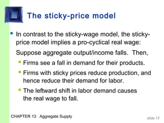
![The sticky-price model
P = s P + (1 − s )[ P + a( Y −Y )]
e
price set by sticky price set by flexible
price firms price firms
Subtract (1−s )P from both sides:
sP = s P e + (1 − s )[ a( Y −Y )]
Divide both sides by s :
(1 − s ) a
P = P e
+ ( Y −Y )
s
CHAPTER 13 Aggregate Supply slide 14](https://image.slidesharecdn.com/chap13-130224055502-phpapp01/85/Chap13-13-320.jpg)


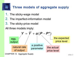
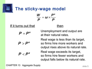
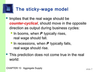
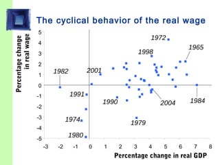
This document provides an overview of key concepts from a chapter on aggregate supply and the short-run tradeoff between inflation and unemployment. It discusses three models of aggregate supply (sticky-wage, imperfect-information, sticky-price) that imply a positive relationship between output and the price level in the short run. It also covers the Phillips curve relationship between inflation and unemployment and how aggregate supply shifts over time as expectations change.