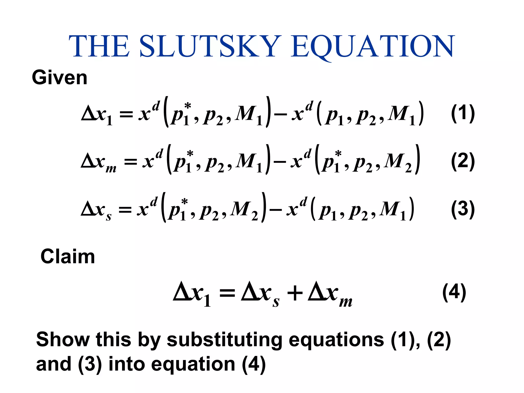
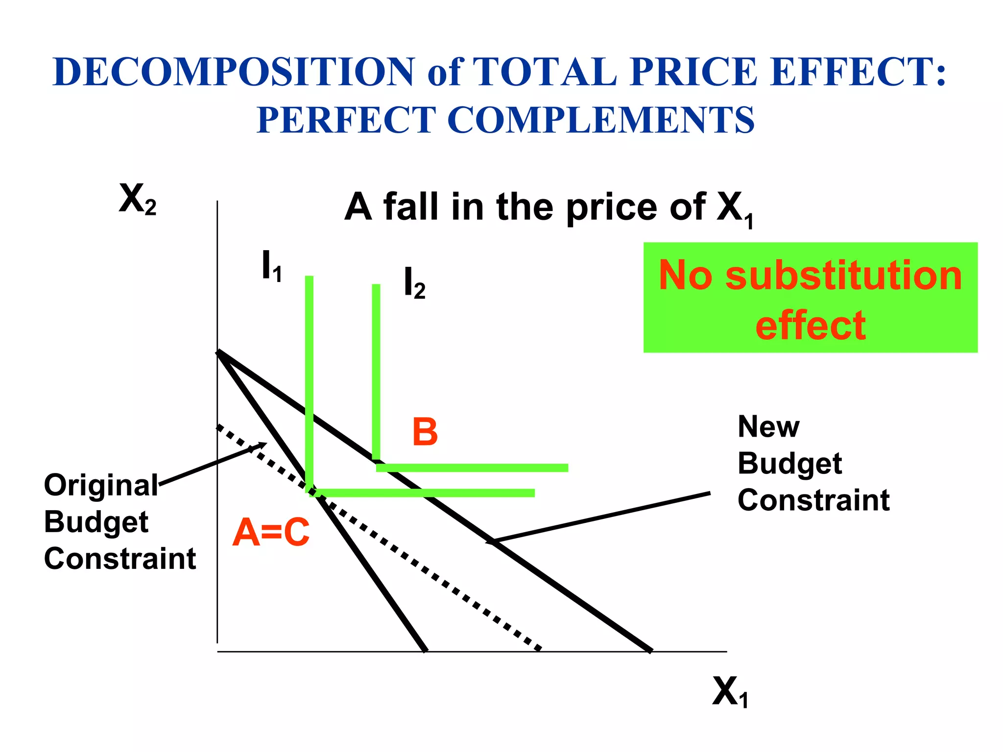
The document discusses the decomposition of the total price effect of a good into substitution and income effects. It explains:
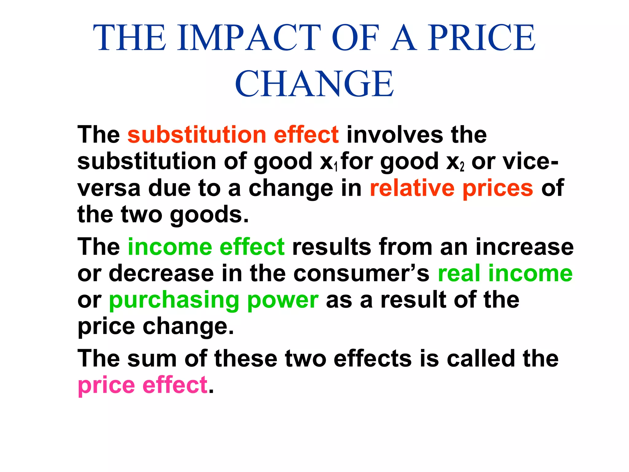
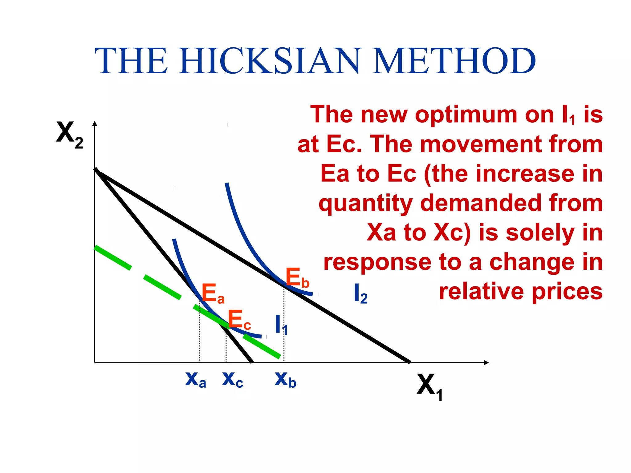
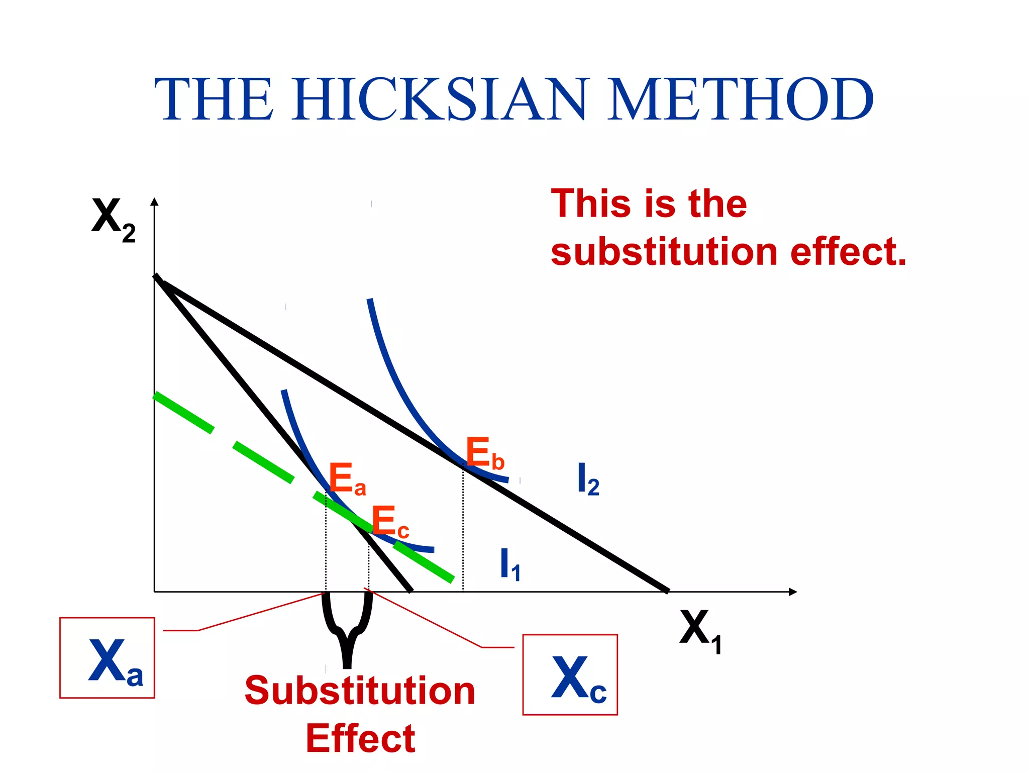
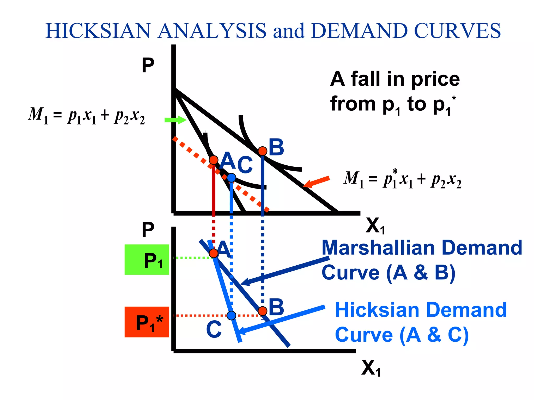
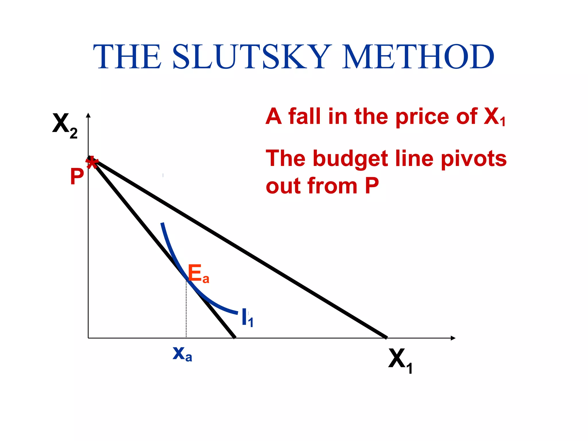
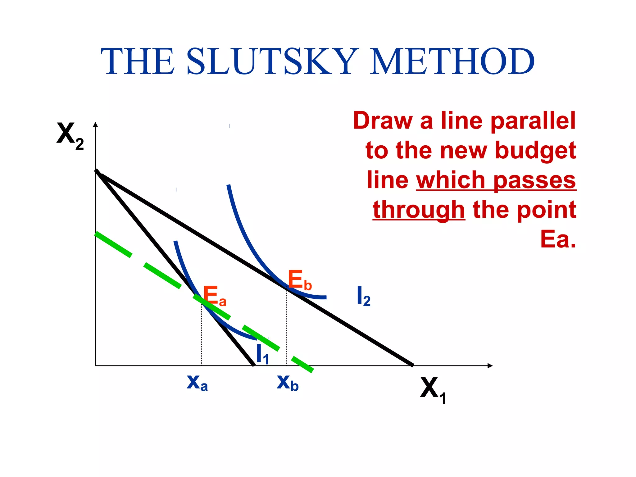
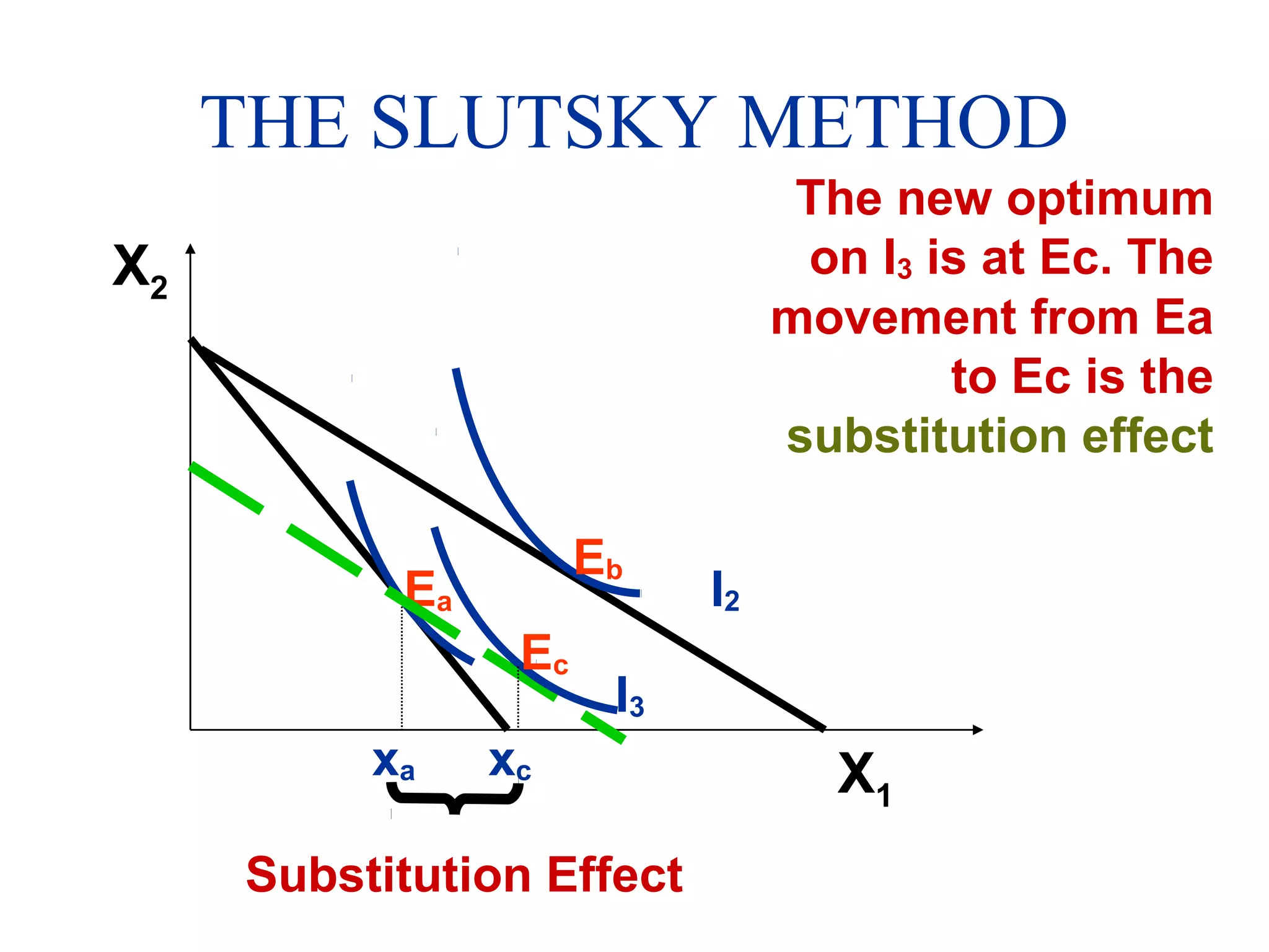
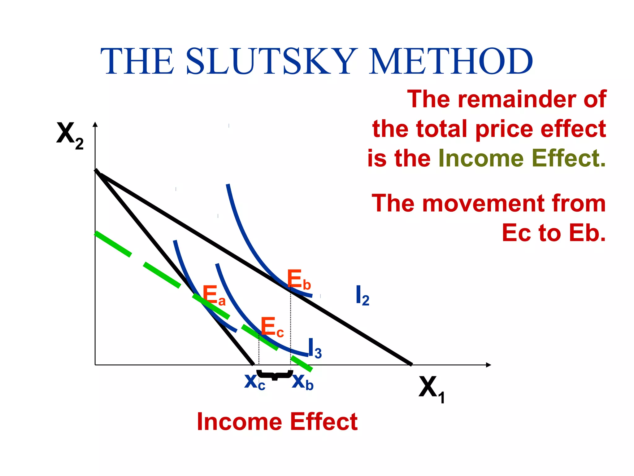
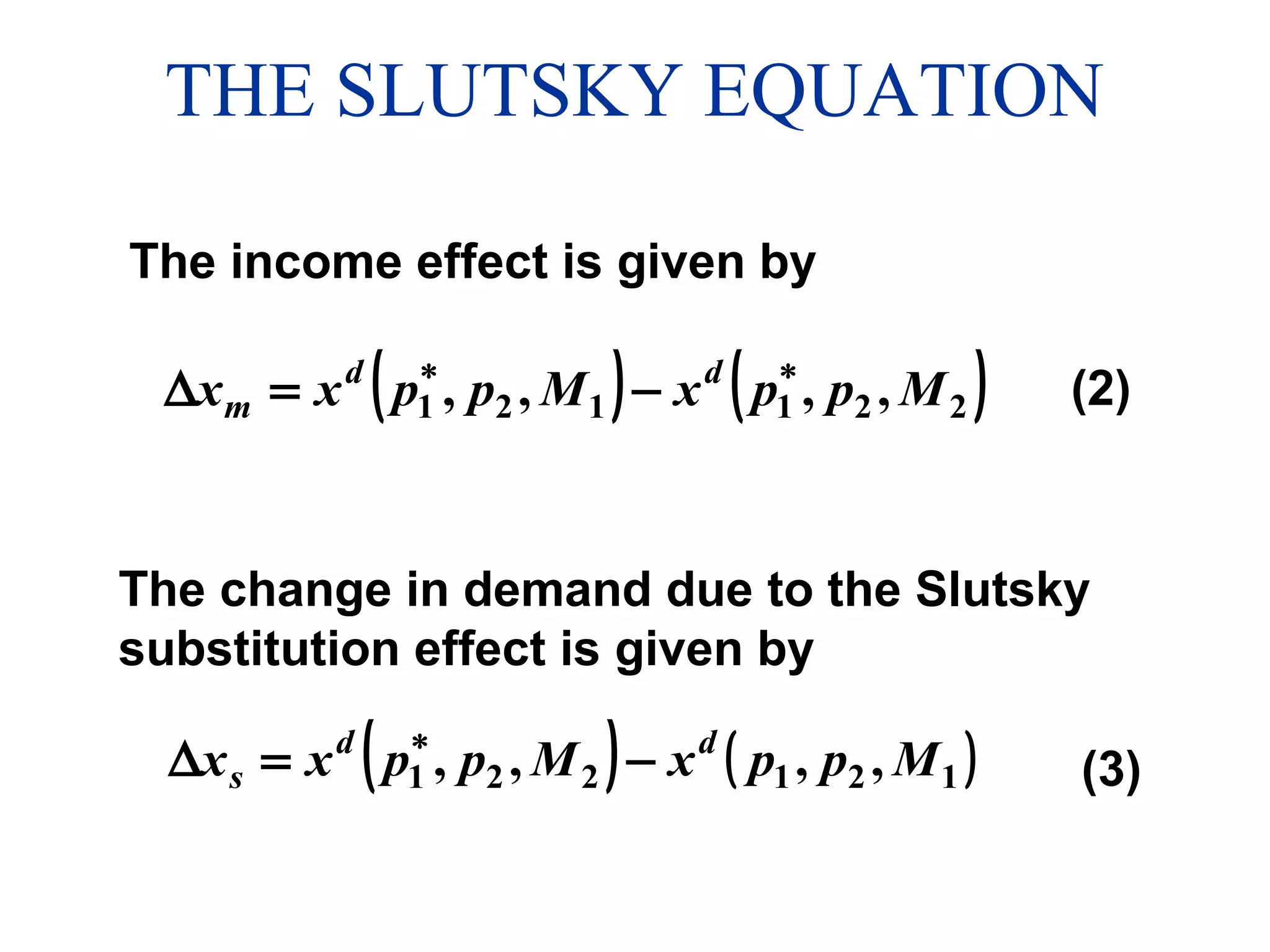
1) The substitution effect captures how consumers change their consumption in response to relative price changes, keeping purchasing power constant. The income effect is due to changes in real income from the price change.
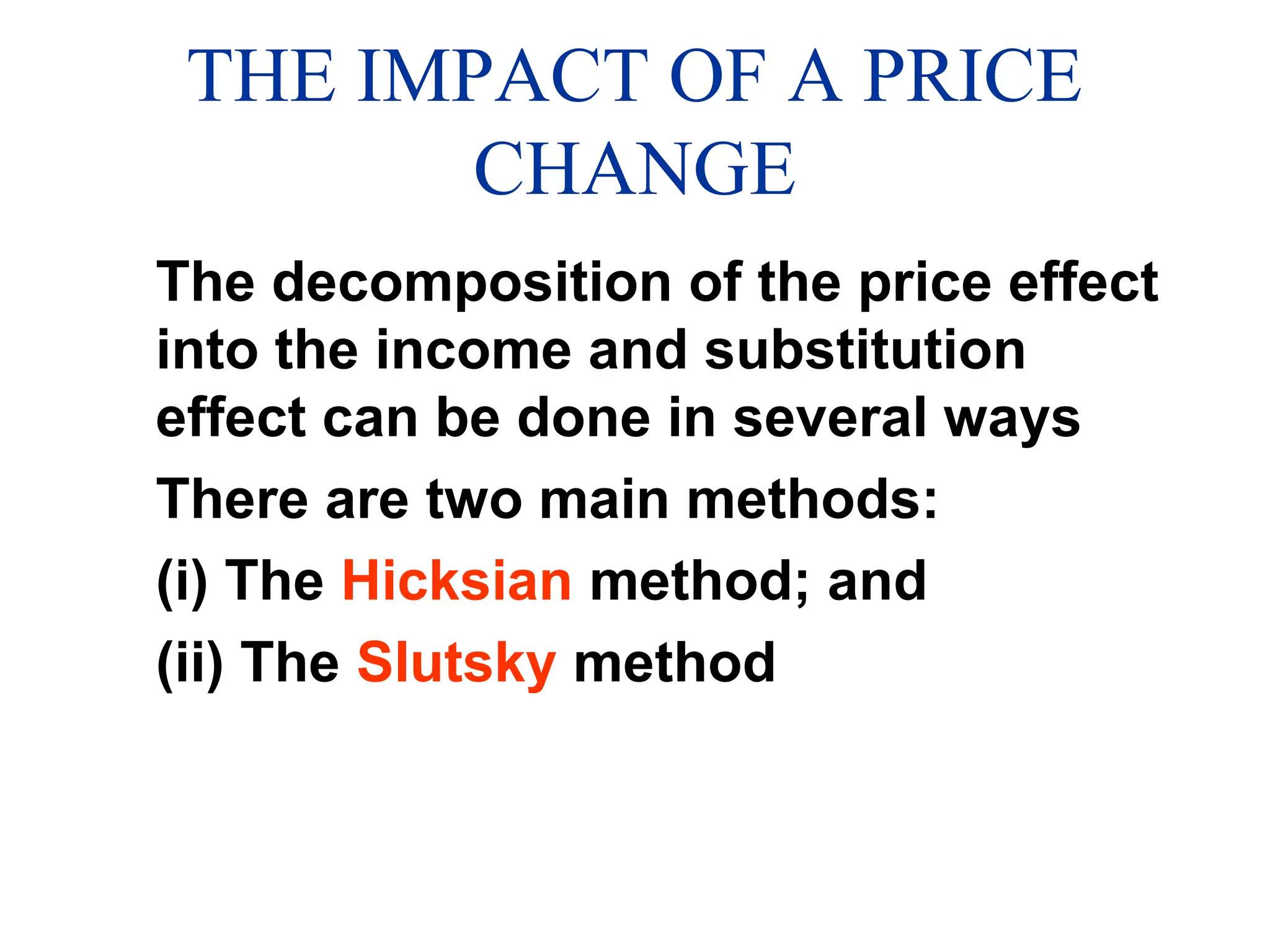
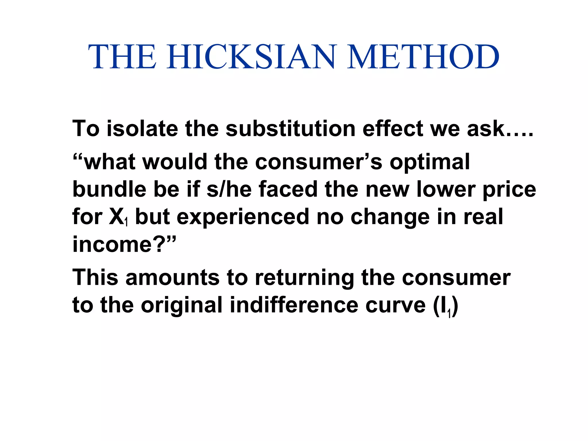
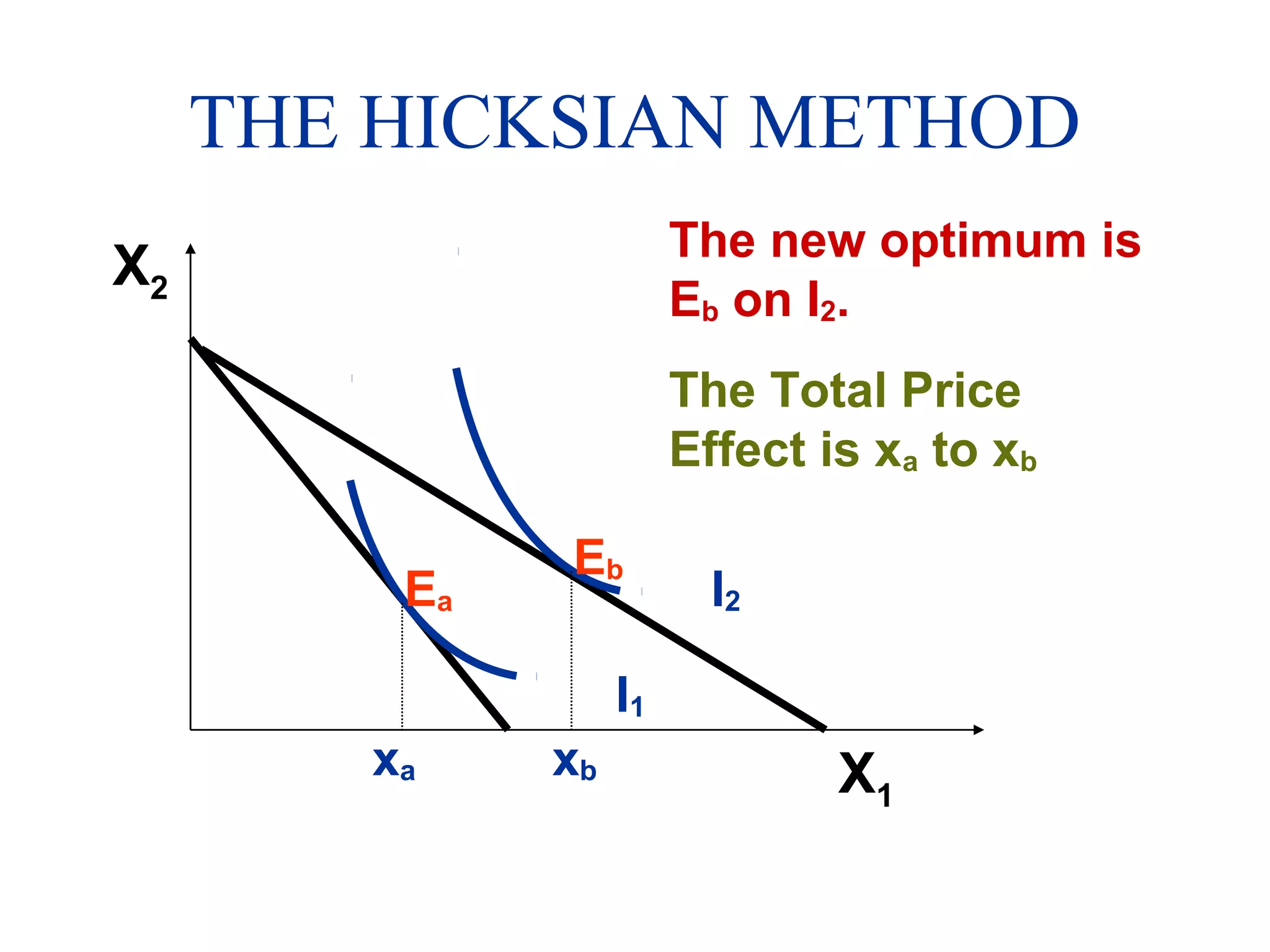
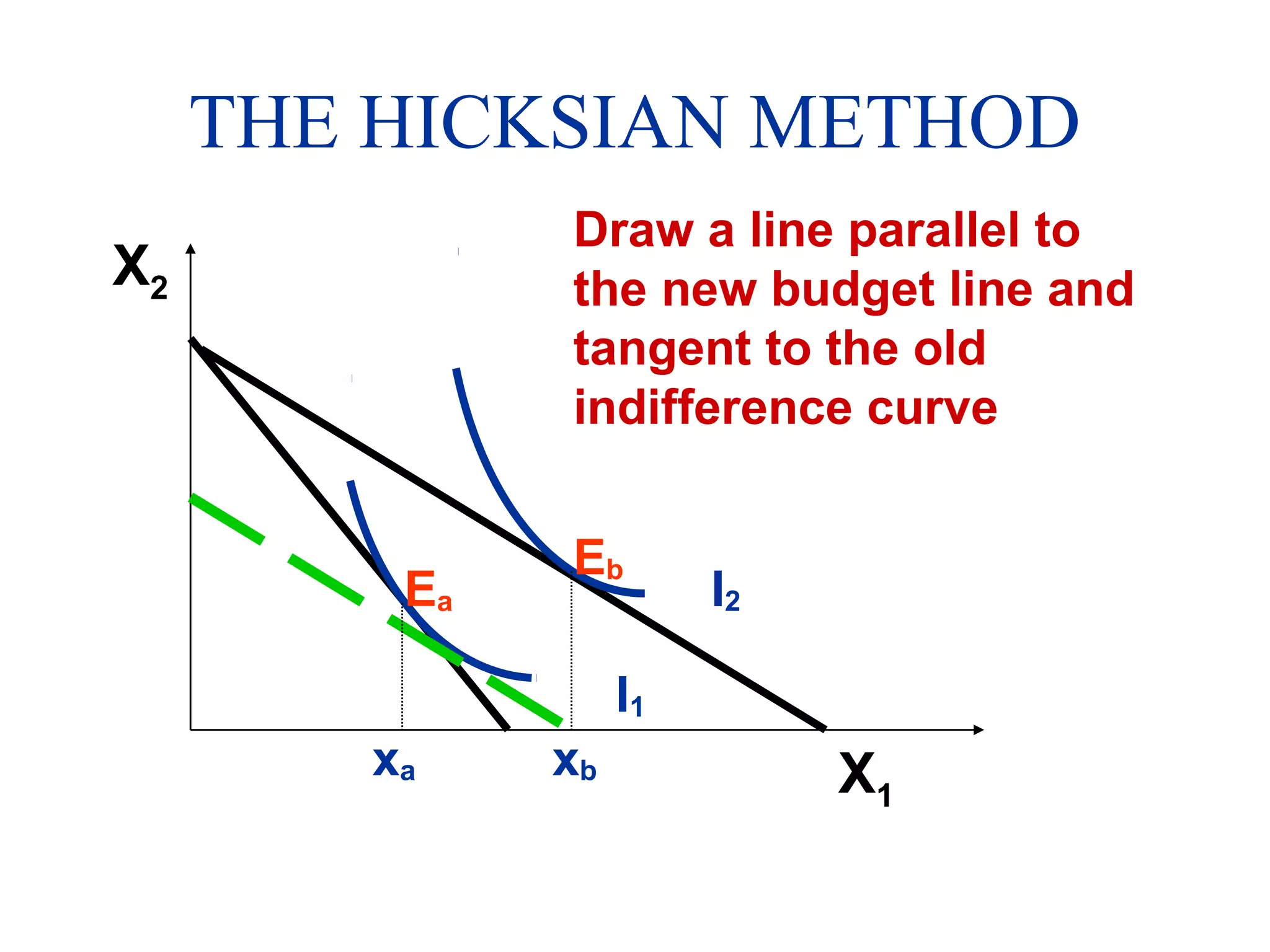
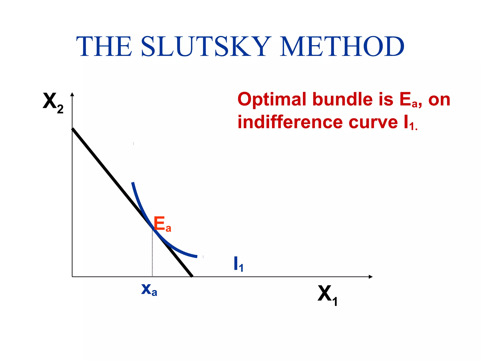
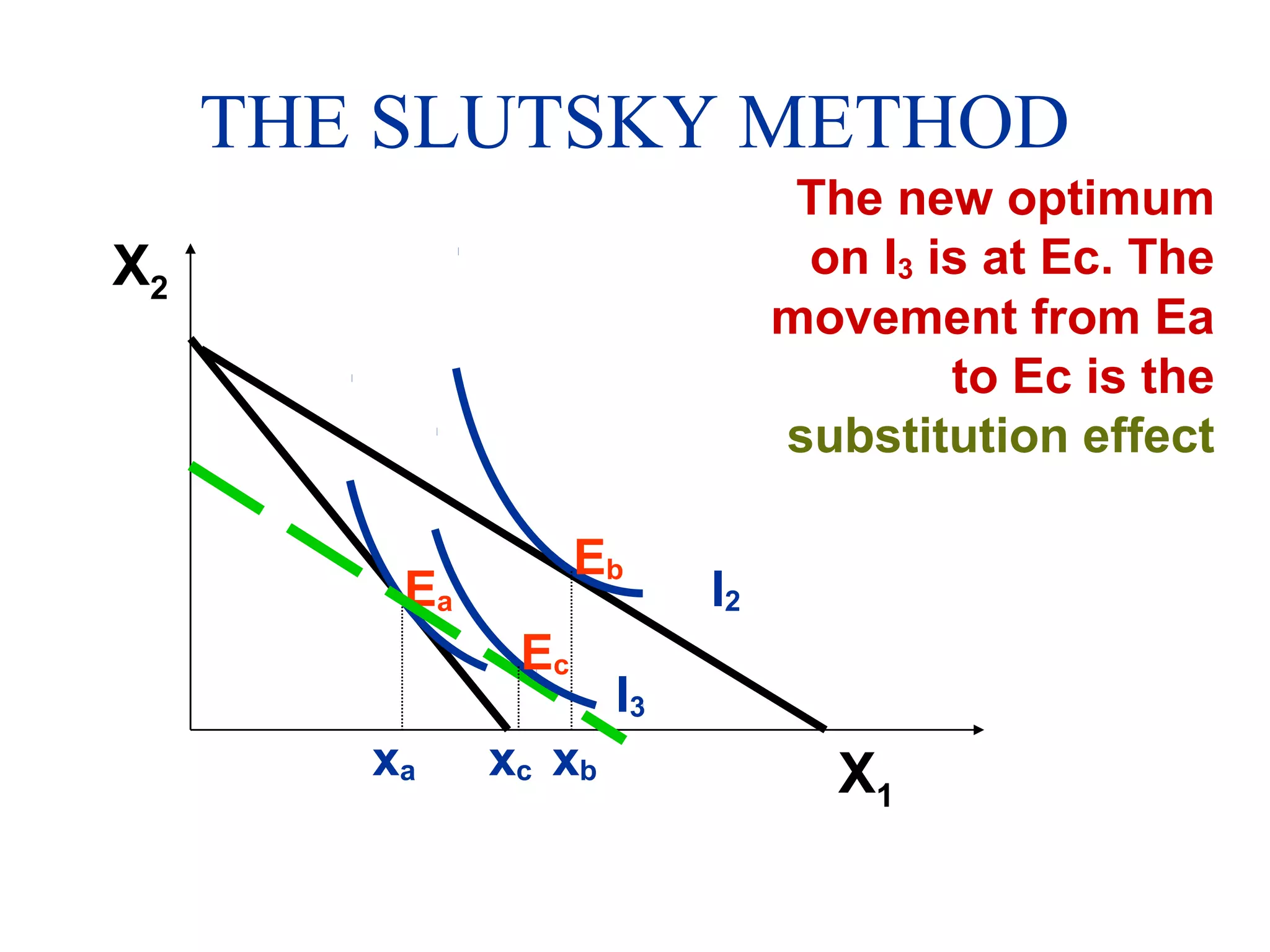
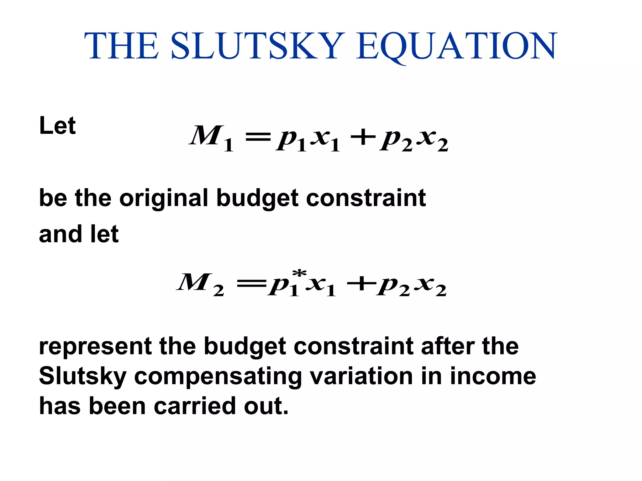
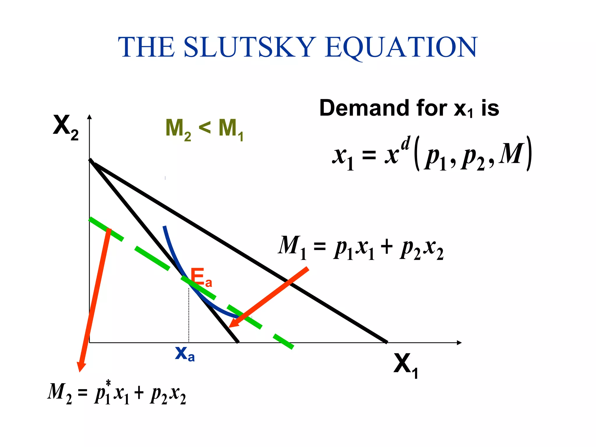
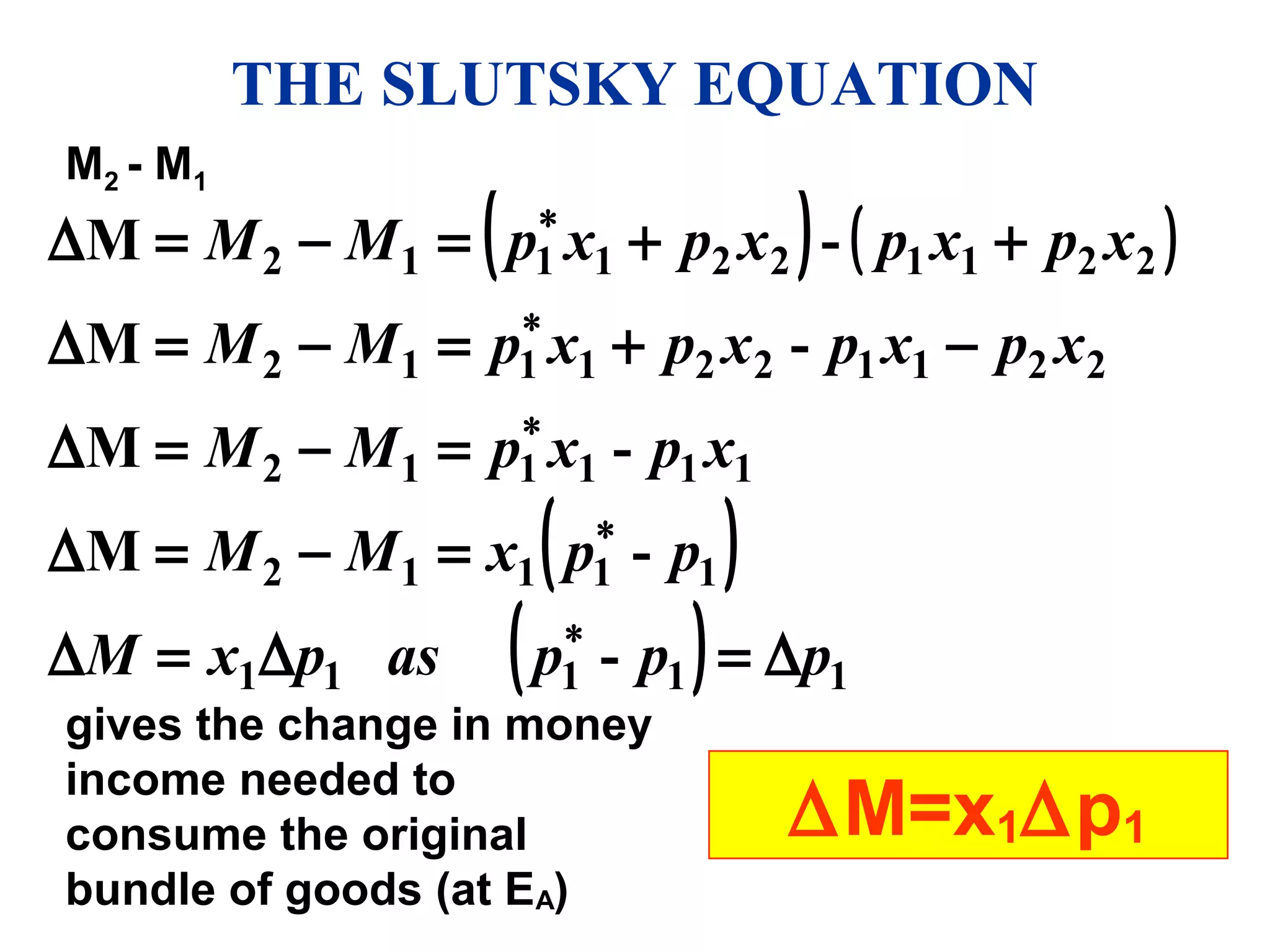
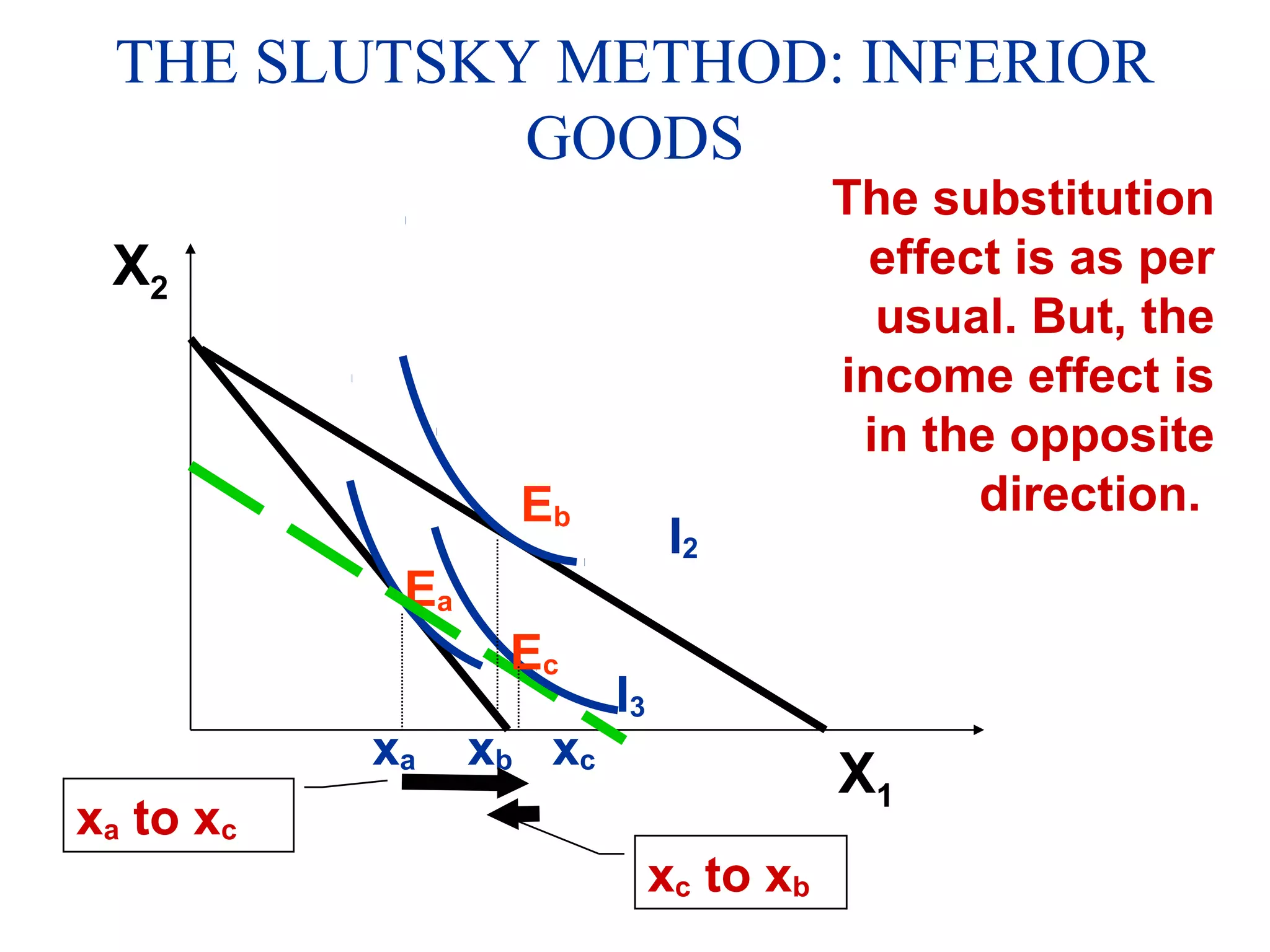
2) Both the Hicksian and Slutsky methods are presented to isolate the substitution and income effects. The Hicksian method involves moving along and between indifference curves. The Slutsky method adjusts income to keep purchasing power constant.
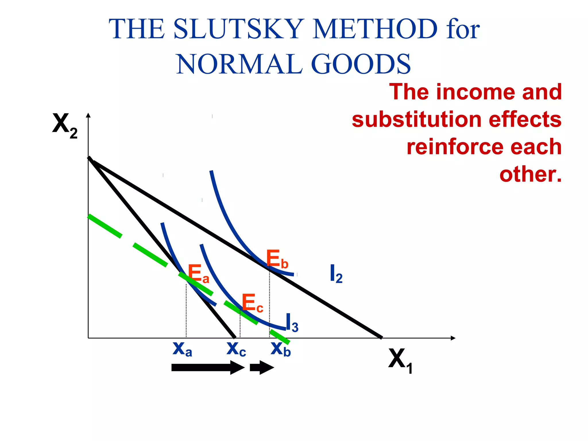
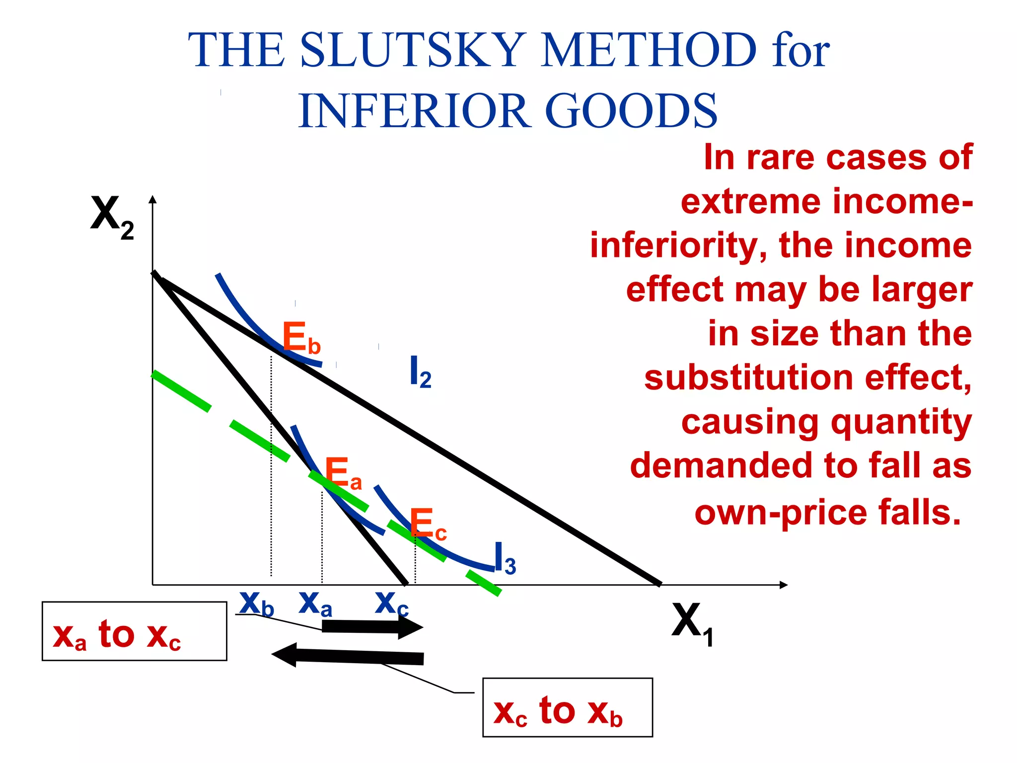
3) For normal goods, the substitution and income effects reinforce each other when the good's own price falls. For inferior goods, they may oppose each


![Working life -_industrial_relations[1]](https://cdn.slidesharecdn.com/ss_thumbnails/workinglife-industrialrelations1-170303212627-thumbnail.jpg?width=640&height=640&fit=bounds)


