The document discusses modeling consumer preferences and indifference curves. It defines preference relations like strict preference, weak preference, and indifference. Indifference curves represent bundles that are equally preferred. They have specific properties like not intersecting and negatively or positively sloped depending on if goods are normal or inferior. The marginal rate of substitution is the slope of the indifference curve and represents the rate at which a consumer is willing to trade one good for another. Well-behaved preferences exhibit properties like monotonicity and convexity.

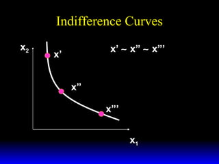
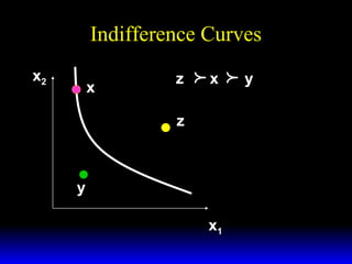
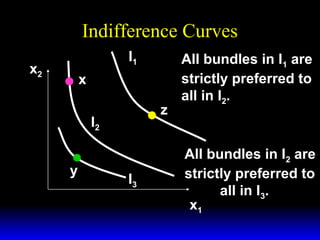
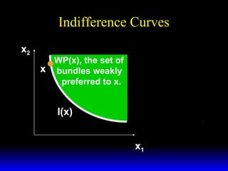
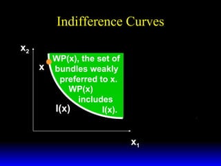
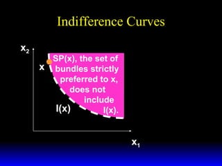
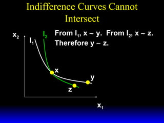
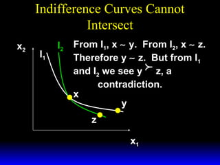
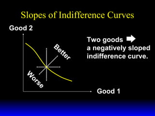
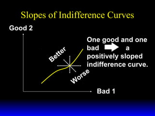
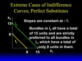
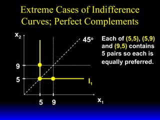
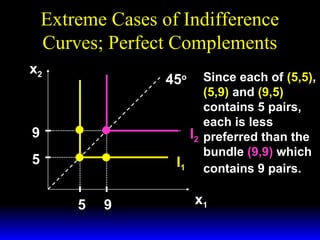
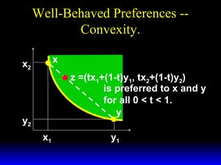
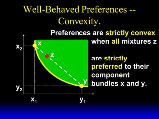
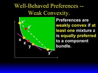
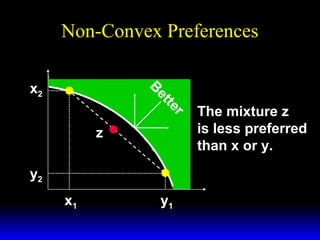
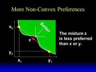
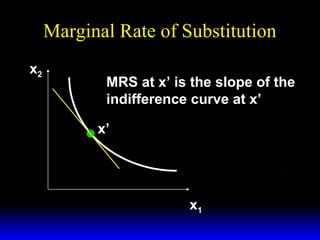
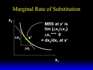
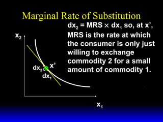
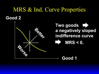
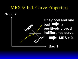
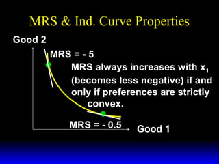
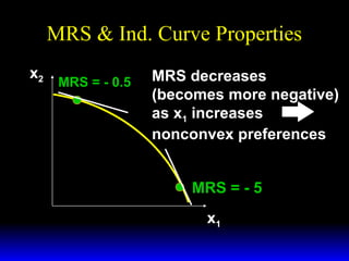
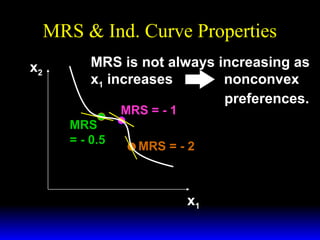
1. Chapter Three
Preferences

2. Rationality in Economics
Behavioral Postulate:
A decisionmaker always chooses its
most preferred alternative from its
set of available alternatives.
So to model choice we must model
decisionmakers’ preferences.

3. Preference Relations
Comparing two different consumption
bundles, x and y:
– strict preference: x is more preferred
than is y.
– weak preference: x is as at least as
preferred as is y.
– indifference: x is exactly as preferred
as is y.

4. Preference Relations
Strict preference, weak preference
and indifference are all preference
relations.
Particularly, they are ordinal
relations; i.e. they state only the
order in which bundles are
preferred.

5. Preference Relations


denotes strict preference;
x y means that bundle x is preferred
strictly to bundle y.

6. Preference Relations


denotes strict preference;
x y means bundle x is preferred
strictly to bundle y.
∼ denotes indifference; x ∼ y means x
and y are equally preferred.

7. Preference Relations


denotes strict preference so
x y means that bundle x is preferred
strictly to bundle y.
∼ denotes indifference; x ∼ y means x
and y are equally preferred.
 denotes weak preference;
~
x  y means x is preferred at least as
~ as is y.
much

8. Preference Relations
x  y and y  x imply x ∼ y.
~
~

9. Preference Relations
x  y and y  x imply x ∼ y.

~
~
x  y and (not y  x) imply x
~
~
y.

10. Assumptions about Preference
Relations
Completeness: For any two bundles
x and y it is always possible to make
the statement that either
x  y
~
or
y  x.
~

11. Assumptions about Preference
Relations
Reflexivity: Any bundle x is always
at least as preferred as itself; i.e.
x
 x.
~

12. Assumptions about Preference
Relations
Transitivity: If
x is at least as preferred as y, and
y is at least as preferred as z, then
x is at least as preferred as z; i.e.
x

~
y and y

~
z
x  z.
~

13. Indifference Curves
Take a reference bundle x’. The set
of all bundles equally preferred to x’
is the indifference curve containing
x’; the set of all bundles y ∼ x’.
Since an indifference “curve” is not
always a curve a better name might
be an indifference “set”.

14. Indifference Curves
x2
x’ ∼ x” ∼ x”’
x’
x”
x”’
x1

15. Indifference Curves

x
z
x
z
y
x1

x2
y

16. Indifference Curves
I1
x2
x
z
I2
y
I3
All bundles in I1 are
strictly preferred to
all in I2.
All bundles in I2 are
strictly preferred to
all in I3.
x1

17. Indifference Curves
x2
WP(x), the set of
x bundles weakly
preferred to x.
I(x)
I(x’)
x1

18. Indifference Curves
x2
WP(x), the set of
x bundles weakly
preferred to x.
WP(x)
includes
I(x)
I(x).
x1

19. Indifference Curves
x2
SP(x), the set of
x bundles strictly
preferred to x,
does not
include
I(x)
I(x).
x1

20. Indifference Curves Cannot
Intersect
x2
I1
I2
From I1, x ∼ y. From I2, x ∼ z.
Therefore y ∼ z.
x
y
z
x1

21. Indifference Curves Cannot
Intersect
I1
I2
From I1, x ∼ y. From I2, x ∼ z.
Therefore y ∼ z. But from I1
and I2 we see y z, a
contradiction.
x
y

x2
z
x1

22. Slopes of Indifference Curves
When more of a commodity is always
preferred, the commodity is a good.
If every commodity is a good then
indifference curves are negatively
sloped.

23. Slopes of Indifference Curves
Good 2
Be
tte
r
W
or
se
Two goods
a negatively sloped
indifference curve.
Good 1

24. Slopes of Indifference Curves
If less of a commodity is always
preferred then the commodity is a
bad.

25. Slopes of Indifference Curves
Good 2
One good and one
bad
a
r
te
positively sloped
et
B
indifference curve.
se
or
W
Bad 1

26. Extreme Cases of Indifference
Curves; Perfect Substitutes
If a consumer always regards units
of commodities 1 and 2 as
equivalent, then the commodities are
perfect substitutes and only the total
amount of the two commodities in
bundles determines their preference
rank-order.

27. Extreme Cases of Indifference
Curves; Perfect Substitutes
x2
15 I2
8
I1
Slopes are constant at - 1.
Bundles in I2 all have a total
of 15 units and are strictly
preferred to all bundles in
I1, which have a total of
only 8 units in them.
x1
8
15

28. Extreme Cases of Indifference
Curves; Perfect Complements
If a consumer always consumes
commodities 1 and 2 in fixed
proportion (e.g. one-to-one), then the
commodities are perfect
complements and only the number of
pairs of units of the two commodities
determines the preference rank-order
of bundles.

29. Extreme Cases of Indifference
Curves; Perfect Complements
x2
45o
9
5
Each of (5,5), (5,9)
and (9,5) contains
5 pairs so each is
equally preferred.
I1
5
9
x1

30. Extreme Cases of Indifference
Curves; Perfect Complements
x2
Since each of (5,5),
(5,9) and (9,5)
contains 5 pairs,
each is less
I2 preferred than the
bundle (9,9) which
I1 contains 9 pairs.
45o
9
5
5
9
x1

31. Preferences Exhibiting Satiation
A bundle strictly preferred to any
other is a satiation point or a bliss
point.
What do indifference curves look like
for preferences exhibiting satiation?

32. Indifference Curves Exhibiting
Satiation
x2
Satiation
(bliss)
point
x1

33. Indifference Curves Exhibiting
Satiation
Be
r tte
tte
e
B
r
Bette
r
x2
x1
Satiation
(bliss)
point

34. Indifference Curves Exhibiting
Satiation
Be
r tte
tte
e
B
r
Bette
r
x2
x1
Satiation
(bliss)
point

35. Indifference Curves for Discrete
Commodities
A commodity is infinitely divisible if
it can be acquired in any quantity;
e.g. water or cheese.
A commodity is discrete if it comes
in unit lumps of 1, 2, 3, … and so on;
e.g. aircraft, ships and refrigerators.

36. Indifference Curves for Discrete
Commodities
Suppose commodity 2 is an infinitely
divisible good (gasoline) while
commodity 1 is a discrete good
(aircraft). What do indifference
“curves” look like?

37. Indifference Curves With a
Discrete Good
Gasoline
Indifference “curves”
are collections of
discrete points.
0
1
2
3
4 Aircraft

38. Well-Behaved Preferences
A preference relation is “wellbehaved” if it is
– monotonic and convex.
Monotonicity: More of any
commodity is always preferred (i.e.
no satiation and every commodity is
a good).

39. Well-Behaved Preferences
Convexity: Mixtures of bundles are
(at least weakly) preferred to the
bundles themselves. E.g., the 50-50
mixture of the bundles x and y is
z = (0.5)x + (0.5)y.
z is at least as preferred as x or y.

40. Well-Behaved Preferences -Convexity.
x
x2
x+
z=
y2
x2+y2
2
is strictly preferred
to both x and y.
y
y2
x1
x1+y1
2
y1

41. Well-Behaved Preferences -Convexity.
x
x2
z =(tx1+(1-t)y1, tx2+(1-t)y2)
is preferred to x and y
for all 0 < t < 1.
y
y2
x1
y1

42. Well-Behaved Preferences -Convexity.
x
x2
Preferences are strictly convex
when all mixtures z
z
y2
x1
are strictly
preferred to their
component
y bundles x and y.
y1

43. Well-Behaved Preferences -Weak Convexity.
Preferences are
weakly convex if at
least one mixture z
is equally preferred
to a component
bundle.
x’
z’
x
z
y
y’

44. Non-Convex Preferences
B
x2
te
et
r
z
y2
x1
y1
The mixture z
is less preferred
than x or y.

45. More Non-Convex Preferences
B
et
x2
r
te
z
y2
x1
y1
The mixture z
is less preferred
than x or y.

46. Slopes of Indifference Curves
The slope of an indifference curve is
its marginal rate-of-substitution
(MRS).
How can a MRS be calculated?

47. Marginal Rate of Substitution
x2
MRS at x’ is the slope of the
indifference curve at x’
x’
x1

48. Marginal Rate of Substitution
x2
∆ x2
x’
MRS at x’ is
lim {∆ x2/∆ x1}
∆ x1
0
= dx2/dx1 at x’
∆ x1
x1

49. Marginal Rate of Substitution
x2
dx2 x’
dx1
dx2 = MRS × dx1 so, at x’,
MRS is the rate at which
the consumer is only just
willing to exchange
commodity 2 for a small
amount of commodity 1.
x1

50. MRS & Ind. Curve Properties
Good 2
r
er
tte
ett
Be
B
Two goods
a negatively sloped
indifference curve
MRS < 0.
se
se
or
or
W
W
Good 1

51. MRS & Ind. Curve Properties
Good 2
er
tt
e
B
One good and one
bad
a
positively sloped
indifference curve
MRS > 0.
se
r
o
W
Bad 1

52. MRS & Ind. Curve Properties
Good 2
MRS = - 5
MRS always increases with x1
(becomes less negative) if and
only if preferences are strictly
convex.
MRS = - 0.5
Good 1

53. MRS & Ind. Curve Properties
x2
MRS = - 0.5
MRS decreases
(becomes more negative)
as x1 increases
nonconvex preferences
MRS = - 5
x1

54. MRS & Ind. Curve Properties
x2
MRS is not always increasing as
x1 increases
nonconvex
preferences.
MRS = - 1
MRS
= - 0.5
MRS = - 2
x1