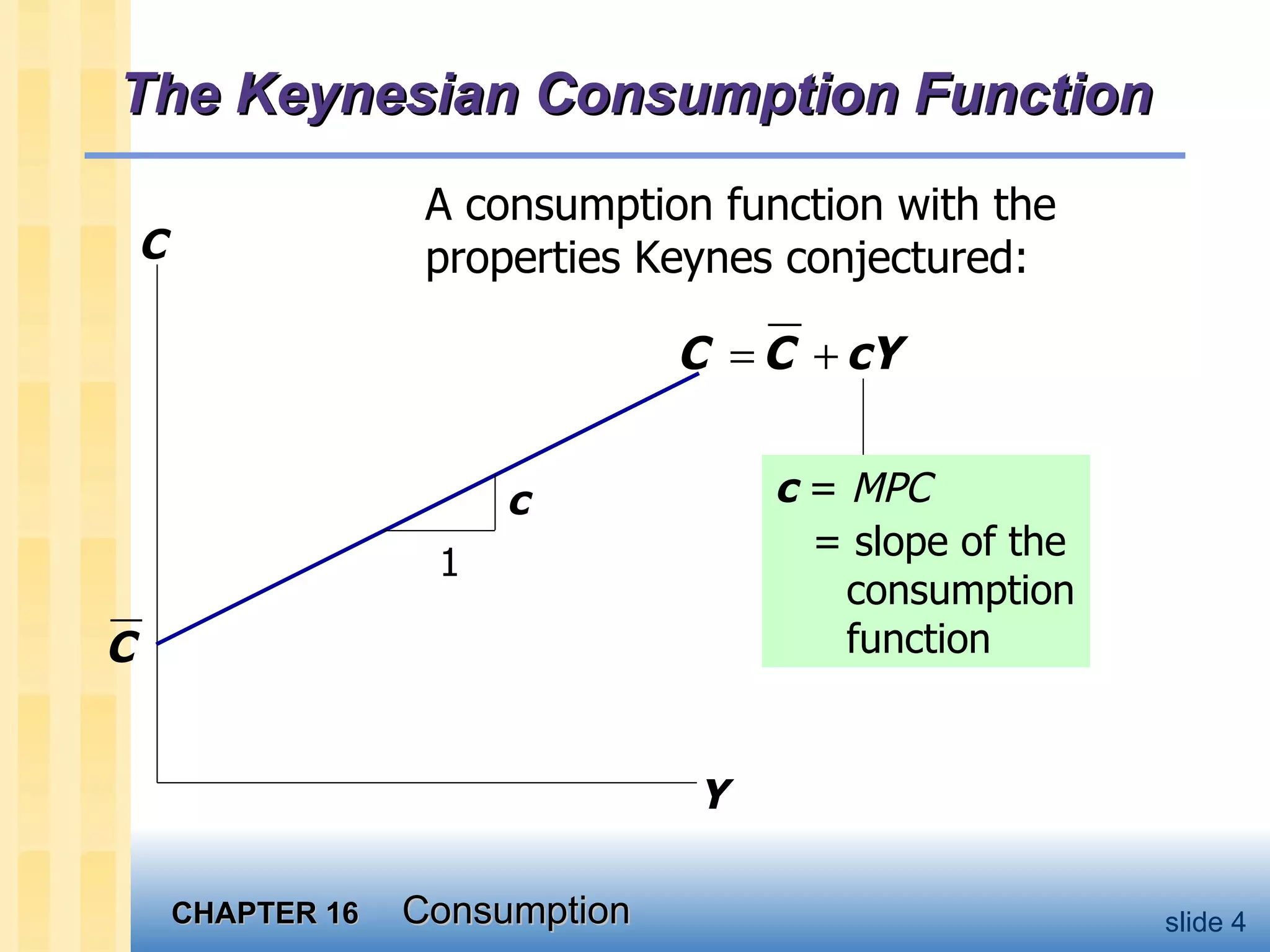
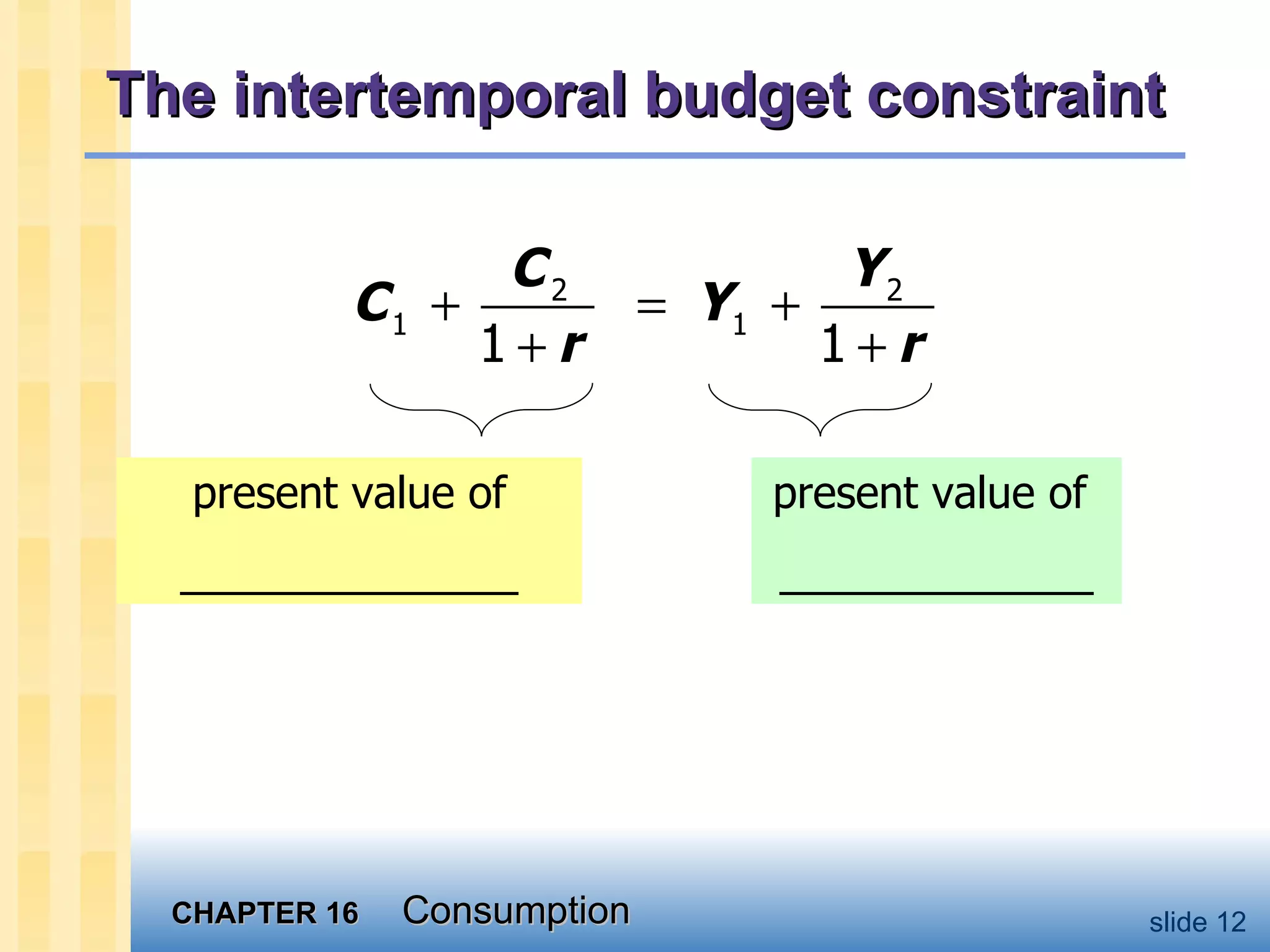
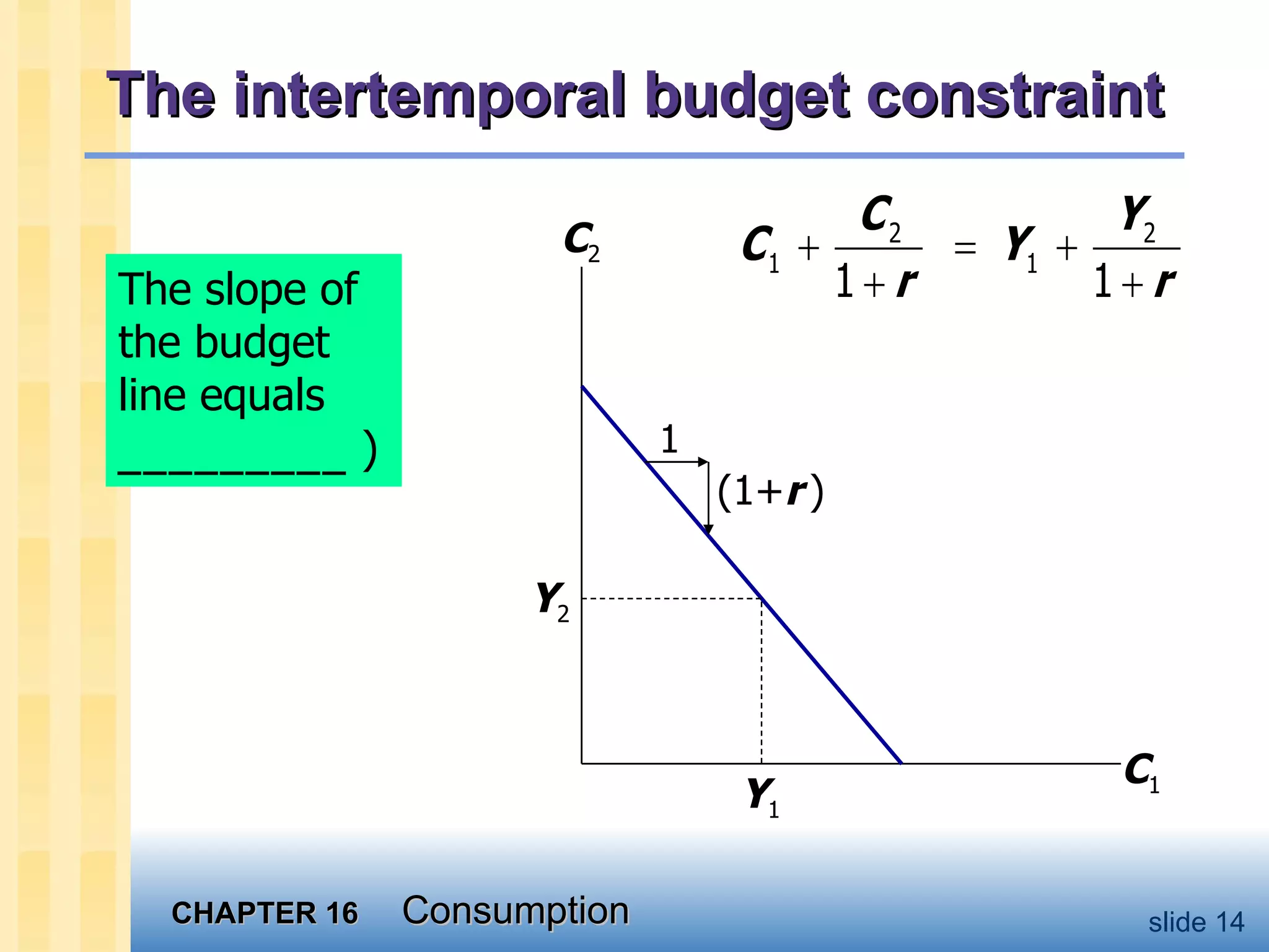
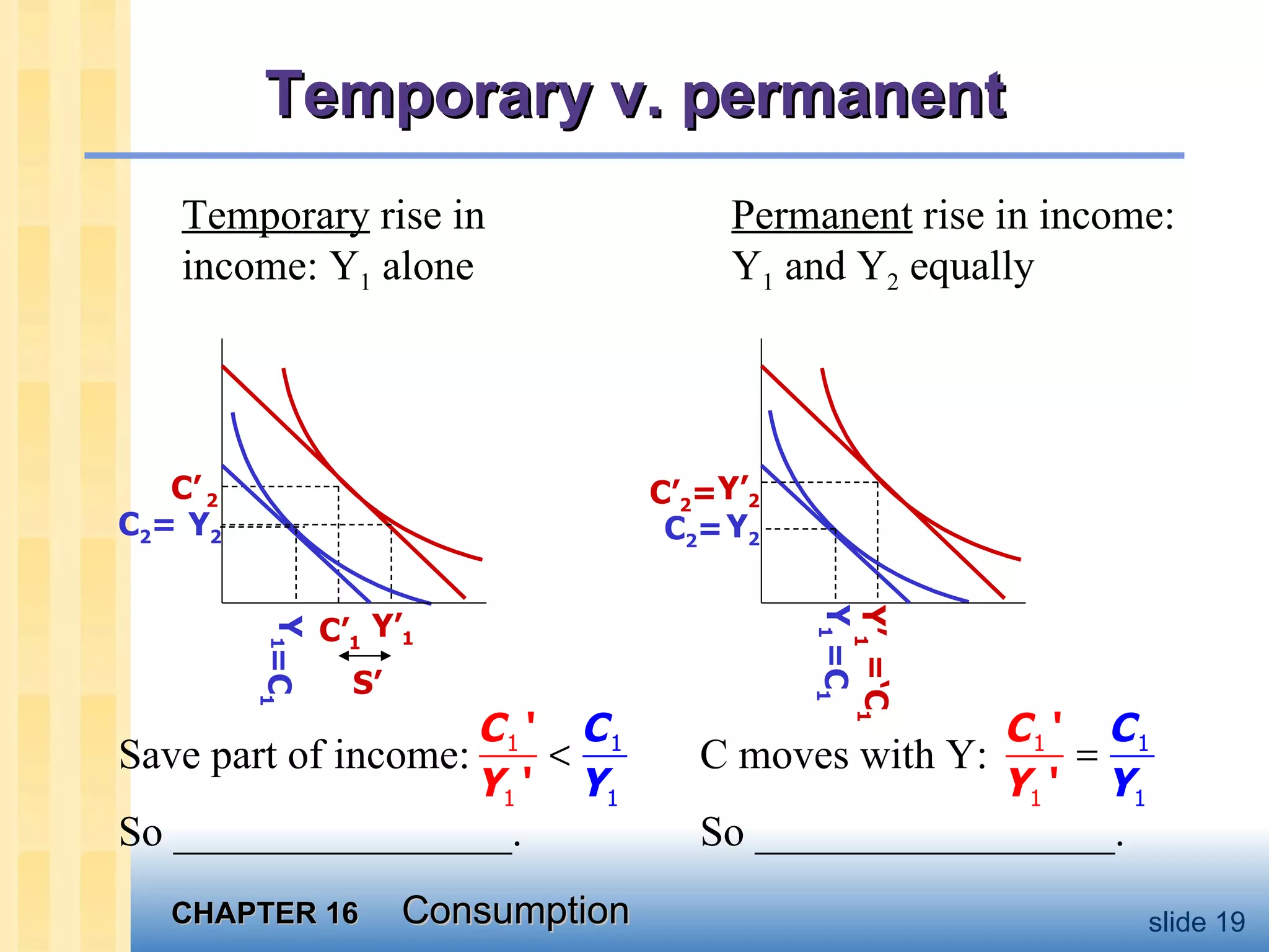
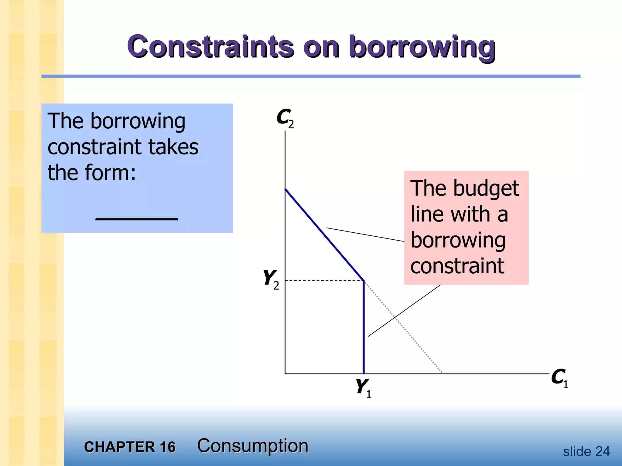
Topic 13: Consumption (chapter 16)  (revised 11/19/03)
Chapter overview This chapter surveys the most prominent work  on consumption: John Maynard Keynes:  consumption and current income Irving Fisher and Intertemporal Choice Franco Modigliani:  the Life-Cycle Hypothesis Milton Friedman:  the Permanent Income Hypothesis Robert Hall:  the Random-Walk Hypothesis David Laibson:  the pull of instant gratification
Keynes’s Conjectures  where  APC   =  average propensity to consume   =  C / Y
The Keynesian Consumption Function A consumption function with the properties Keynes conjectured: C Y 1 c c  =  MPC = slope of the consumption function
The Keynesian Consumption Function As income rises, the APC falls (consumers save a bigger fraction of their income). C Y slope =  APC
Early Empirical Successes:  Results from Early Studies Households with higher incomes:    MPC  > 0    MPC  < 1    APC      as  Y    Very strong correlation between income and consumption       income seemed to be the main    determinant of consumption
Problems for the  Keynesian Consumption Function Based on the Keynesian consumption function, economists predicted that  __________ _________________________________. This prediction did not come true: As incomes grew, the APC did not fall,  and  C   grew just as fast. Simon Kuznets showed that  C / Y   was  very stable in long time series data.
The Consumption Puzzle C Y Consumption function from long time series data (constant  APC  ) Consumption function from cross-sectional household data  (falling  APC  )
Irving Fisher and Intertemporal Choice The basis for much subsequent work on consumption.  Assumes consumer is forward-looking and chooses consumption for the present and future to maximize lifetime satisfaction. Consumer’s choices are subject to an  ___________________________ ,  a measure of the total resources available for present and future consumption
The basic two-period model Period 1:  the present Period 2:  the future Notation Y 1  is income in period 1 Y 2  is income in period 2 C 1  is consumption in period 1 C 2  is consumption in period 2 S  =  Y 1      C 1  is ______________ ( S  < 0 if the consumer borrows in period 1)
Deriving the  intertemporal budget constraint Period 2 budget constraint: Rearrange to put  C   terms on one side  and  Y   terms on the other: Finally, divide through by (1+ r   ):
The intertemporal budget constraint present value of ______________ present value of  _____________
The budget constraint shows all combinations  of  C 1  and  C 2  that just exhaust the consumer’s resources. The intertemporal budget constraint C 1 C 2 Y 1 Y 2 _______ _____ Consump = income in both periods
The slope of the budget line equals     ) The intertemporal budget constraint C 1 C 2 Y 1 Y 2 1 (1+ r   )
An  ________ ______ shows all combinations of  C 1  and  C 2  that make the consumer __________________________. Consumer preferences Higher indifference curves represent higher levels of happiness. Y Z X W C 1 C 2 IC 1 IC 2
Marginal rate of substitution  ( MRS   ):  the amount of  C 2  consumer would be ________________ _________________. Consumer preferences The slope of an indifference curve at any point equals the  MRS   at that point. So the MRS is the (negative) of the ___________________________. C 1 C 2 IC 1 1 MRS
The optimal ( C 1 , C 2 ) is where the budget line just touches the highest indifference curve.  Optimization At the optimal point,  __________ C 1 C 2 O
An increase in  Y 1  or   Y 2   shifts the budget line outward.  How  C   responds to changes in   Y   Results:  Provided they are both normal goods,  C 1  and  C 2  both increase, … _______________________________________________________.  C 1 C 2
Temporary v. permanent Temporary  rise in income: Y 1  alone Permanent  rise in income: Y 1  and Y 2  equally S’ Y 2 Save part of income: So ________________. C moves with Y: So _________________. C 2 = C’ 1 C’  2 C’ 2 = =‘C 1 =C 1 C 2 = =C 1 Y 1 Y 2 Y 1 Y’ 1 Y’ 2 Y’ 1
Keynes vs. Fisher Keynes:  current consumption depends only on current income Fisher:  current consumption depends only on  ________________________________;  the timing of income is irrelevant  because the consumer can borrow or lend between periods.
An increase in  r  pivots the budget line around the  point ( Y 1 , Y 2   ).  How  C   responds to changes in   r As depicted here,  ______________ . However, it could turn out differently… A C 1 C 2 Y 1 Y 2 A B
How  C   responds to changes in   r ___________ If consumer is a saver, the rise in  r   makes him better off, which tends to increase consumption in both periods. ____________ The rise in  r   increases the opportunity cost of current consumption, which tends to reduce  C 1  and increase  C 2 .  Both effects   C 2 .  Whether  C 1  rises or falls depends on the relative size of the income & substitution effects.
Constraints on borrowing In Fisher’s theory, the timing of income is irrelevant because the consumer can borrow and lend across periods.  Example:  If consumer learns that her future income will increase, she can spread the extra consumption over both periods by borrowing in the current period.  However, if consumer faces  _______________  (aka “liquidity constraints”), then she may not be able to increase current consumption and her consumption may behave as in the Keynesian theory even though she is rational & forward-looking
The borrowing constraint takes the form: ______ Constraints on borrowing Y 1 Y 2 C 1 C 2 The budget line with a borrowing constraint
The borrowing constraint is not binding if the consumer’s  optimal  C 1   ___________. Consumer optimization when the borrowing constraint is  not binding Y 1 C 1 C 2
The optimal choice is at point D.  But since the consumer cannot borrow, the best he can do is point E. Consumer optimization when the borrowing constraint  is binding Y 1 D E C 1 C 2
So under borrowing constraints, current consumption __________ __________ __________. Suppose increase in income in period 1 E Y’ 1 =C 1 ’ The rise in income to Y’ 1  shifts the budget constraint right. C’ 1  rises with Y’ 1. Y 1 =C 1 C 1 C 2
due to Franco Modigliani (1950s) Fisher’s model says that consumption depends on lifetime income, and people try to achieve smooth consumption.  The LCH says that _________ __________ over the phases of the consumer’s “life cycle,” and saving allows the consumer to achieve smooth consumption.  The Life-Cycle Hypothesis
The Life-Cycle Hypothesis The basic model: W  = Y  =  (assumed constant) R  = number of years until retirement T  = lifetime in years Assumptions:  zero real interest rate (for simplicity) consumption-smoothing is optimal
The Life-Cycle Hypothesis Lifetime resources = To achieve smooth consumption, consumer divides her resources equally over time: C  = _____________ , or C   =   W  +    Y   where    = (1/ T  ) is the marginal propensity to  consume out of wealth     = ( R / T  ) is the marginal propensity to consume out of income
Implications of the Life-Cycle Hypothesis The Life-Cycle Hypothesis can solve the consumption puzzle:  The  APC   implied by the life-cycle consumption function is C / Y  =     Across households, wealth does not vary as much as income, so high income households _______________________ than low income households. Over time, aggregate wealth and income grow together, causing APC __________.
Implications of the Life-Cycle Hypothesis The LCH implies that saving varies systematically over a person’s lifetime. Saving Dissaving Retirement  begins End  of life Consumption Income $ Wealth
Numerical Example Suppose you start working at age 20, work until age 65, and expert to earn $50,000 each year, and you expect to live to 80. Lifetime income =  Spread over 60 years, so C = So need to save $12,500 per year.
Example continued Suppose you win a lottery which gives you $1000 today.  Will spread it out over all T years, so consumption rises by only  $1000/T = $16.70 this year. So temporary rise in income has a _____ ____________. But if lottery gives you $1000 every year for the T years, consumption rises by ________ _________ this year.
The Permanent Income Hypothesis due to Milton Friedman (1957) The PIH views current income  Y   as the sum of two components:  _______________  Y  P   (average income, which people expect to persist into the future) _______________  Y  T (temporary deviations from average income)
Consumers use saving & borrowing to smooth consumption in response to transitory changes in income.  The PIH consumption function: C   = where     is the fraction of permanent income that people consume per year.  The Permanent Income Hypothesis
The PIH can solve the consumption puzzle: The PIH implies APC  =  C/Y   = To the extent that high income households have higher transitory income than low income households, the APC will be _____ _________________ income households.  Over the long run, income variation is due mainly if not solely to variation in permanent income, which implies a __________.  The Permanent Income Hypothesis
PIH vs. LCH In both, people try to achieve smooth consumption in the face of changing current income. In the LCH, current income changes systematically as people move through their life cycle. In the PIH, current income is subject to random, transitory fluctuations.  Both hypotheses can explain the consumption puzzle.
The Random-Walk Hypothesis due to Robert Hall (1978) based on Fisher’s model & PIH, in which forward-looking consumers base consumption on expected future income Hall adds the assumption of  rational expectations , that people use all available information to forecast future variables like income.
The Random-Walk Hypothesis If PIH is correct and consumers have rational expectations, then consumption should follow a  random walk :  ________________________ _____________________. A change in income or wealth that was anticipated has already been factored into expected permanent income, so it will not change consumption.  Only unanticipated changes in income or wealth that alter expected permanent income will change consumption.
If consumers obey the PIH  and have rational expectations, then policy changes  will affect consumption  only if _________________.  Implication of the R-W Hypothesis
The Psychology of Instant Gratification Theories from Fisher to Hall assumes that consumers are rational and act to maximize lifetime utility. recent studies by David Laibson and others consider the psychology of consumers.
The Psychology of Instant Gratification Consumers consider themselves to be imperfect decision-makers. E.g., in one survey, 76% said they were not saving enough for retirement. Laibson:  The “pull of instant gratification” explains why people don’t save as much as a perfectly rational lifetime utility maximizer would save.
Two Questions and Time Inconsistency 1. Would you prefer   (A)  a candy today, or   (B) two candies tomorrow? 2.  Would you prefer  (A) a candy in 100 days, or    (B)  two candies in 101 days? In studies, most people answered A to question 1, and B to question 2.  A person confronted with question 2 may choose B.  100 days later, when he is confronted with question 1, the pull of instant gratification may induce him to change his mind.
Summing up Recall simple Keynesian consumption function: where only current income (Y) mattered. Research shows other things should be included:  expected future income  (perm’t income model) wealth  (life cycle model) interest rates  (Fisher model) but  current income  should still be present (due to borrowing constraints) Modern policy analysis models allow for all this.

MACROECONOMICS-CH16

  • 1.
    Topic 13: Consumption(chapter 16) (revised 11/19/03)
  • 2.
    Chapter overview Thischapter surveys the most prominent work on consumption: John Maynard Keynes: consumption and current income Irving Fisher and Intertemporal Choice Franco Modigliani: the Life-Cycle Hypothesis Milton Friedman: the Permanent Income Hypothesis Robert Hall: the Random-Walk Hypothesis David Laibson: the pull of instant gratification
  • 3.
    Keynes’s Conjectures where APC = average propensity to consume = C / Y
  • 4.
    The Keynesian ConsumptionFunction A consumption function with the properties Keynes conjectured: C Y 1 c c = MPC = slope of the consumption function
  • 5.
    The Keynesian ConsumptionFunction As income rises, the APC falls (consumers save a bigger fraction of their income). C Y slope = APC
  • 6.
    Early Empirical Successes: Results from Early Studies Households with higher incomes:  MPC > 0  MPC < 1  APC  as Y  Very strong correlation between income and consumption  income seemed to be the main determinant of consumption
  • 7.
    Problems for the Keynesian Consumption Function Based on the Keynesian consumption function, economists predicted that __________ _________________________________. This prediction did not come true: As incomes grew, the APC did not fall, and C grew just as fast. Simon Kuznets showed that C / Y was very stable in long time series data.
  • 8.
    The Consumption PuzzleC Y Consumption function from long time series data (constant APC ) Consumption function from cross-sectional household data (falling APC )
  • 9.
    Irving Fisher andIntertemporal Choice The basis for much subsequent work on consumption. Assumes consumer is forward-looking and chooses consumption for the present and future to maximize lifetime satisfaction. Consumer’s choices are subject to an ___________________________ , a measure of the total resources available for present and future consumption
  • 10.
    The basic two-periodmodel Period 1: the present Period 2: the future Notation Y 1 is income in period 1 Y 2 is income in period 2 C 1 is consumption in period 1 C 2 is consumption in period 2 S = Y 1  C 1 is ______________ ( S < 0 if the consumer borrows in period 1)
  • 11.
    Deriving the intertemporal budget constraint Period 2 budget constraint: Rearrange to put C terms on one side and Y terms on the other: Finally, divide through by (1+ r ):
  • 12.
    The intertemporal budgetconstraint present value of ______________ present value of _____________
  • 13.
    The budget constraintshows all combinations of C 1 and C 2 that just exhaust the consumer’s resources. The intertemporal budget constraint C 1 C 2 Y 1 Y 2 _______ _____ Consump = income in both periods
  • 14.
    The slope ofthe budget line equals  ) The intertemporal budget constraint C 1 C 2 Y 1 Y 2 1 (1+ r )
  • 15.
    An ______________ shows all combinations of C 1 and C 2 that make the consumer __________________________. Consumer preferences Higher indifference curves represent higher levels of happiness. Y Z X W C 1 C 2 IC 1 IC 2
  • 16.
    Marginal rate ofsubstitution ( MRS ): the amount of C 2 consumer would be ________________ _________________. Consumer preferences The slope of an indifference curve at any point equals the MRS at that point. So the MRS is the (negative) of the ___________________________. C 1 C 2 IC 1 1 MRS
  • 17.
    The optimal (C 1 , C 2 ) is where the budget line just touches the highest indifference curve. Optimization At the optimal point, __________ C 1 C 2 O
  • 18.
    An increase in Y 1 or Y 2 shifts the budget line outward. How C responds to changes in Y Results: Provided they are both normal goods, C 1 and C 2 both increase, … _______________________________________________________. C 1 C 2
  • 19.
    Temporary v. permanentTemporary rise in income: Y 1 alone Permanent rise in income: Y 1 and Y 2 equally S’ Y 2 Save part of income: So ________________. C moves with Y: So _________________. C 2 = C’ 1 C’ 2 C’ 2 = =‘C 1 =C 1 C 2 = =C 1 Y 1 Y 2 Y 1 Y’ 1 Y’ 2 Y’ 1
  • 20.
    Keynes vs. FisherKeynes: current consumption depends only on current income Fisher: current consumption depends only on ________________________________; the timing of income is irrelevant because the consumer can borrow or lend between periods.
  • 21.
    An increase in r pivots the budget line around the point ( Y 1 , Y 2 ). How C responds to changes in r As depicted here, ______________ . However, it could turn out differently… A C 1 C 2 Y 1 Y 2 A B
  • 22.
    How C responds to changes in r ___________ If consumer is a saver, the rise in r makes him better off, which tends to increase consumption in both periods. ____________ The rise in r increases the opportunity cost of current consumption, which tends to reduce C 1 and increase C 2 . Both effects  C 2 . Whether C 1 rises or falls depends on the relative size of the income & substitution effects.
  • 23.
    Constraints on borrowingIn Fisher’s theory, the timing of income is irrelevant because the consumer can borrow and lend across periods. Example: If consumer learns that her future income will increase, she can spread the extra consumption over both periods by borrowing in the current period. However, if consumer faces _______________ (aka “liquidity constraints”), then she may not be able to increase current consumption and her consumption may behave as in the Keynesian theory even though she is rational & forward-looking
  • 24.
    The borrowing constrainttakes the form: ______ Constraints on borrowing Y 1 Y 2 C 1 C 2 The budget line with a borrowing constraint
  • 25.
    The borrowing constraintis not binding if the consumer’s optimal C 1 ___________. Consumer optimization when the borrowing constraint is not binding Y 1 C 1 C 2
  • 26.
    The optimal choiceis at point D. But since the consumer cannot borrow, the best he can do is point E. Consumer optimization when the borrowing constraint is binding Y 1 D E C 1 C 2
  • 27.
    So under borrowingconstraints, current consumption __________ __________ __________. Suppose increase in income in period 1 E Y’ 1 =C 1 ’ The rise in income to Y’ 1 shifts the budget constraint right. C’ 1 rises with Y’ 1. Y 1 =C 1 C 1 C 2
  • 28.
    due to FrancoModigliani (1950s) Fisher’s model says that consumption depends on lifetime income, and people try to achieve smooth consumption. The LCH says that _________ __________ over the phases of the consumer’s “life cycle,” and saving allows the consumer to achieve smooth consumption. The Life-Cycle Hypothesis
  • 29.
    The Life-Cycle HypothesisThe basic model: W = Y = (assumed constant) R = number of years until retirement T = lifetime in years Assumptions: zero real interest rate (for simplicity) consumption-smoothing is optimal
  • 30.
    The Life-Cycle HypothesisLifetime resources = To achieve smooth consumption, consumer divides her resources equally over time: C = _____________ , or C =  W +  Y where  = (1/ T ) is the marginal propensity to consume out of wealth  = ( R / T ) is the marginal propensity to consume out of income
  • 31.
    Implications of theLife-Cycle Hypothesis The Life-Cycle Hypothesis can solve the consumption puzzle: The APC implied by the life-cycle consumption function is C / Y =  Across households, wealth does not vary as much as income, so high income households _______________________ than low income households. Over time, aggregate wealth and income grow together, causing APC __________.
  • 32.
    Implications of theLife-Cycle Hypothesis The LCH implies that saving varies systematically over a person’s lifetime. Saving Dissaving Retirement begins End of life Consumption Income $ Wealth
  • 33.
    Numerical Example Supposeyou start working at age 20, work until age 65, and expert to earn $50,000 each year, and you expect to live to 80. Lifetime income = Spread over 60 years, so C = So need to save $12,500 per year.
  • 34.
    Example continued Supposeyou win a lottery which gives you $1000 today. Will spread it out over all T years, so consumption rises by only $1000/T = $16.70 this year. So temporary rise in income has a _____ ____________. But if lottery gives you $1000 every year for the T years, consumption rises by ________ _________ this year.
  • 35.
    The Permanent IncomeHypothesis due to Milton Friedman (1957) The PIH views current income Y as the sum of two components: _______________ Y P (average income, which people expect to persist into the future) _______________ Y T (temporary deviations from average income)
  • 36.
    Consumers use saving& borrowing to smooth consumption in response to transitory changes in income. The PIH consumption function: C = where  is the fraction of permanent income that people consume per year. The Permanent Income Hypothesis
  • 37.
    The PIH cansolve the consumption puzzle: The PIH implies APC = C/Y = To the extent that high income households have higher transitory income than low income households, the APC will be _____ _________________ income households. Over the long run, income variation is due mainly if not solely to variation in permanent income, which implies a __________. The Permanent Income Hypothesis
  • 38.
    PIH vs. LCHIn both, people try to achieve smooth consumption in the face of changing current income. In the LCH, current income changes systematically as people move through their life cycle. In the PIH, current income is subject to random, transitory fluctuations. Both hypotheses can explain the consumption puzzle.
  • 39.
    The Random-Walk Hypothesisdue to Robert Hall (1978) based on Fisher’s model & PIH, in which forward-looking consumers base consumption on expected future income Hall adds the assumption of rational expectations , that people use all available information to forecast future variables like income.
  • 40.
    The Random-Walk HypothesisIf PIH is correct and consumers have rational expectations, then consumption should follow a random walk : ________________________ _____________________. A change in income or wealth that was anticipated has already been factored into expected permanent income, so it will not change consumption. Only unanticipated changes in income or wealth that alter expected permanent income will change consumption.
  • 41.
    If consumers obeythe PIH and have rational expectations, then policy changes will affect consumption only if _________________. Implication of the R-W Hypothesis
  • 42.
    The Psychology ofInstant Gratification Theories from Fisher to Hall assumes that consumers are rational and act to maximize lifetime utility. recent studies by David Laibson and others consider the psychology of consumers.
  • 43.
    The Psychology ofInstant Gratification Consumers consider themselves to be imperfect decision-makers. E.g., in one survey, 76% said they were not saving enough for retirement. Laibson: The “pull of instant gratification” explains why people don’t save as much as a perfectly rational lifetime utility maximizer would save.
  • 44.
    Two Questions andTime Inconsistency 1. Would you prefer (A) a candy today, or (B) two candies tomorrow? 2. Would you prefer (A) a candy in 100 days, or (B) two candies in 101 days? In studies, most people answered A to question 1, and B to question 2. A person confronted with question 2 may choose B. 100 days later, when he is confronted with question 1, the pull of instant gratification may induce him to change his mind.
  • 45.
    Summing up Recallsimple Keynesian consumption function: where only current income (Y) mattered. Research shows other things should be included: expected future income (perm’t income model) wealth (life cycle model) interest rates (Fisher model) but current income should still be present (due to borrowing constraints) Modern policy analysis models allow for all this.

Editor's Notes

  • #2 This long chapter is a survey of the most prominent work on consumption since Keynes. After reviewing the Keynesian consumption function and its implications, the chapter presents Irving Fisher’s theory of intertemporal choice, the basis for much subsequent work on consumption. The chapter presents the Life-Cycle and Permanent Income Hypotheses, then discusses Hall’s Random Walk Hypothesis. Finally, there is a brief discussion of some very recent work by Laibson and others on psychology and economics, in particular how the pull of instant gratification can cause consumers to deviate from perfect rationality.