This document provides an overview of key concepts related to risky assets and portfolio choice including:
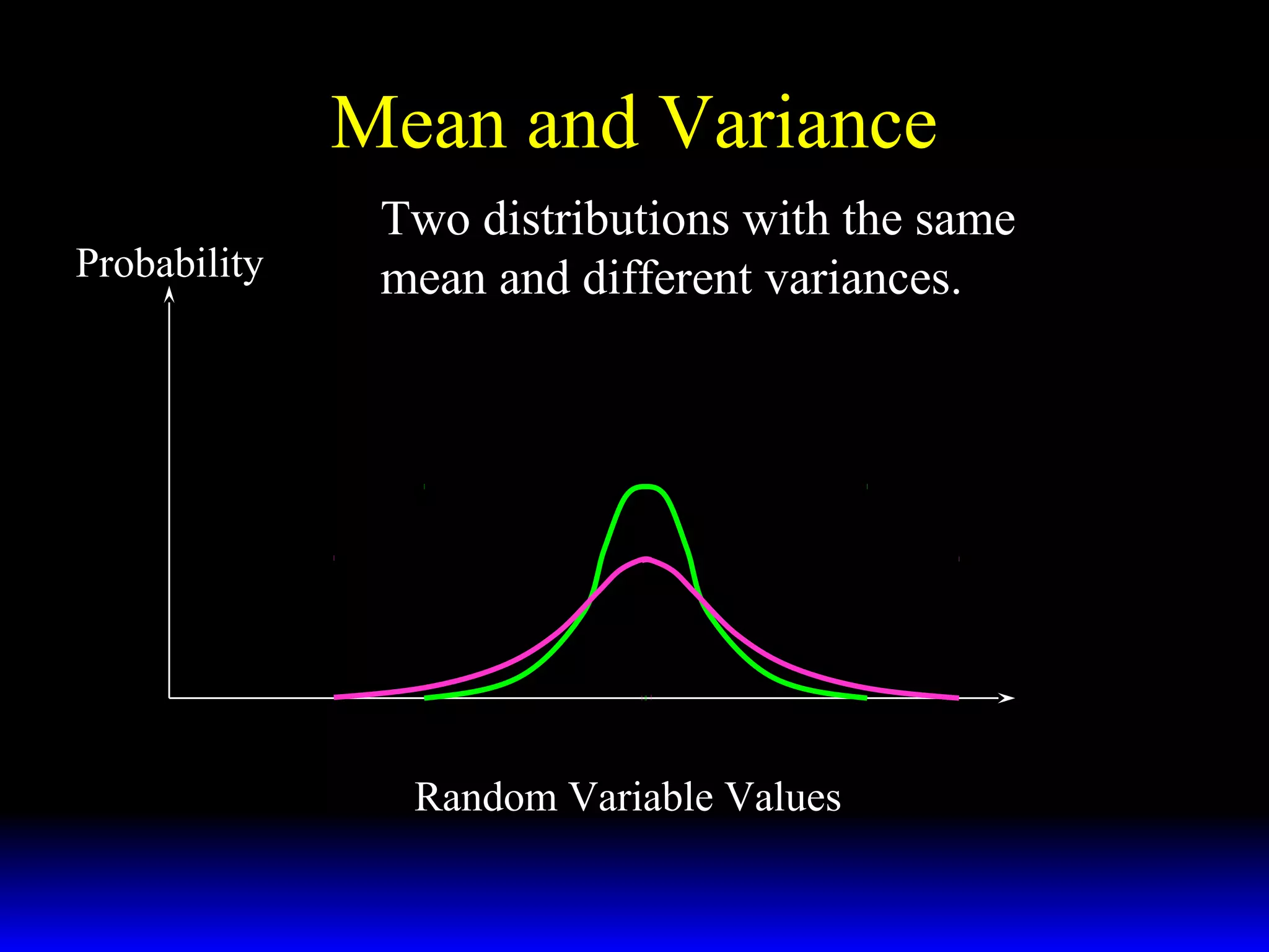
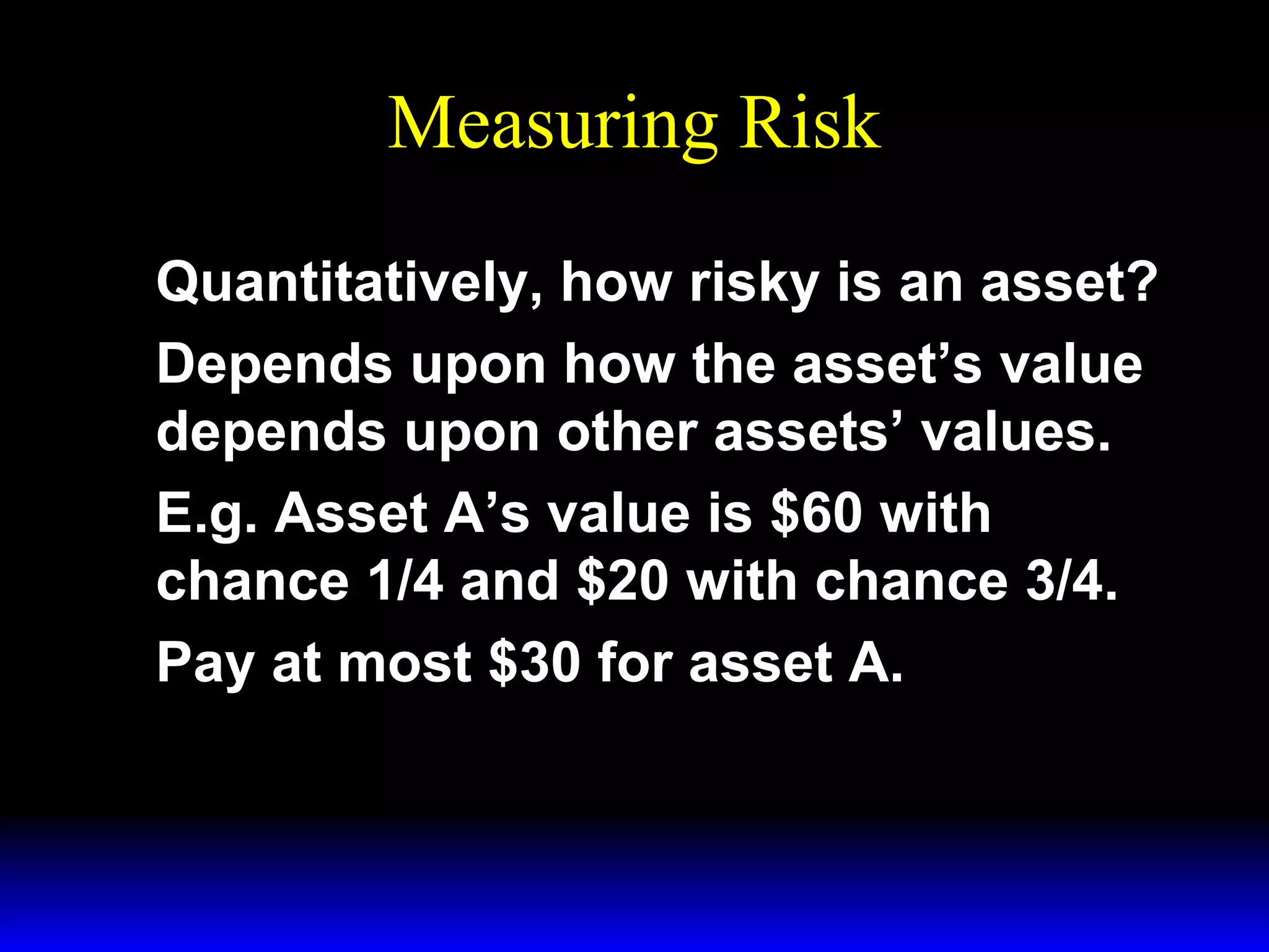
- The mean and variance of distributions and how they measure the expected value and variation of random variables.
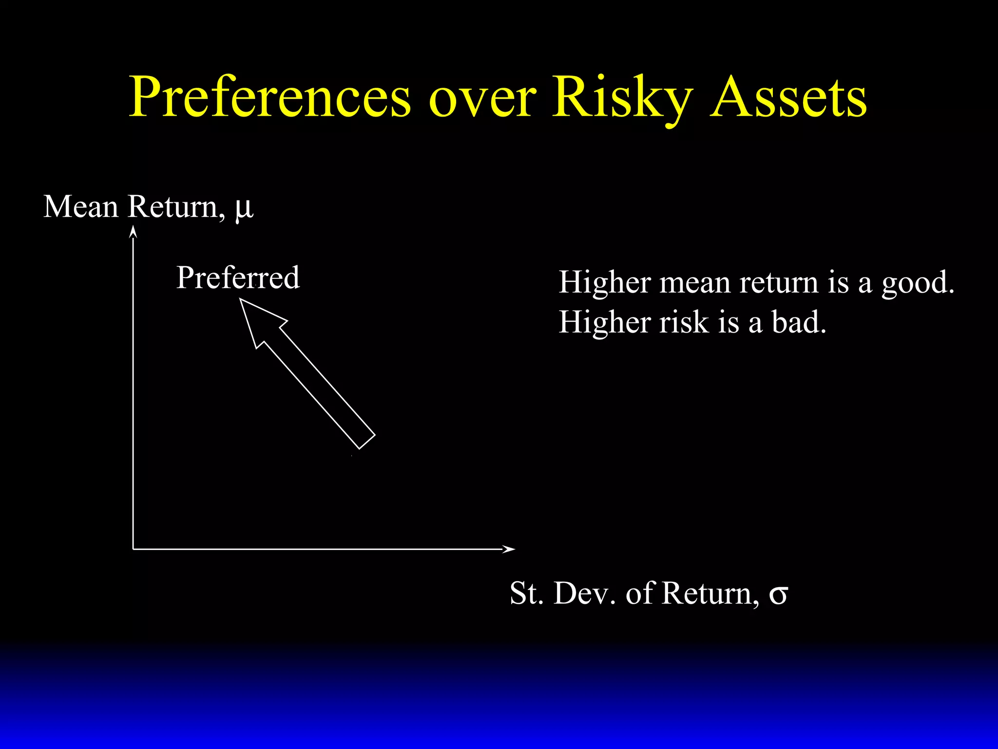
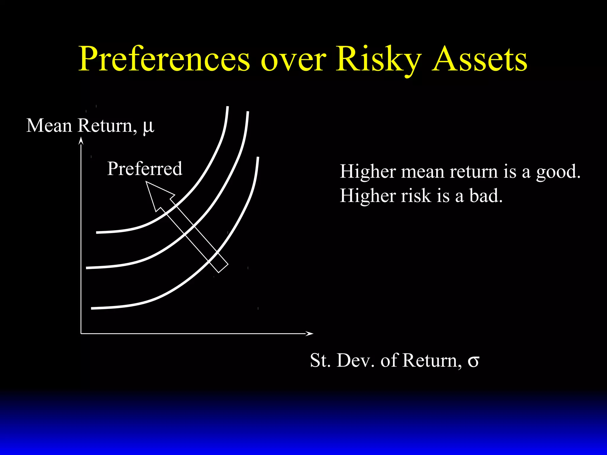
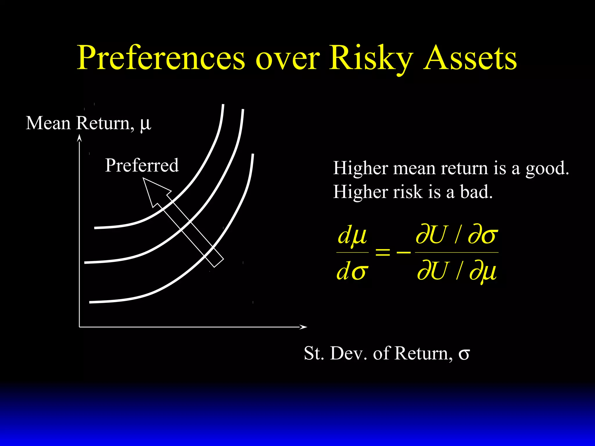
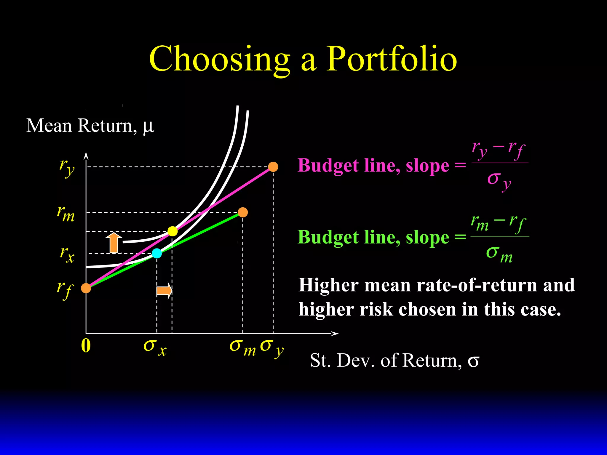
- How investors prefer higher returns but less risk, represented by a utility function.
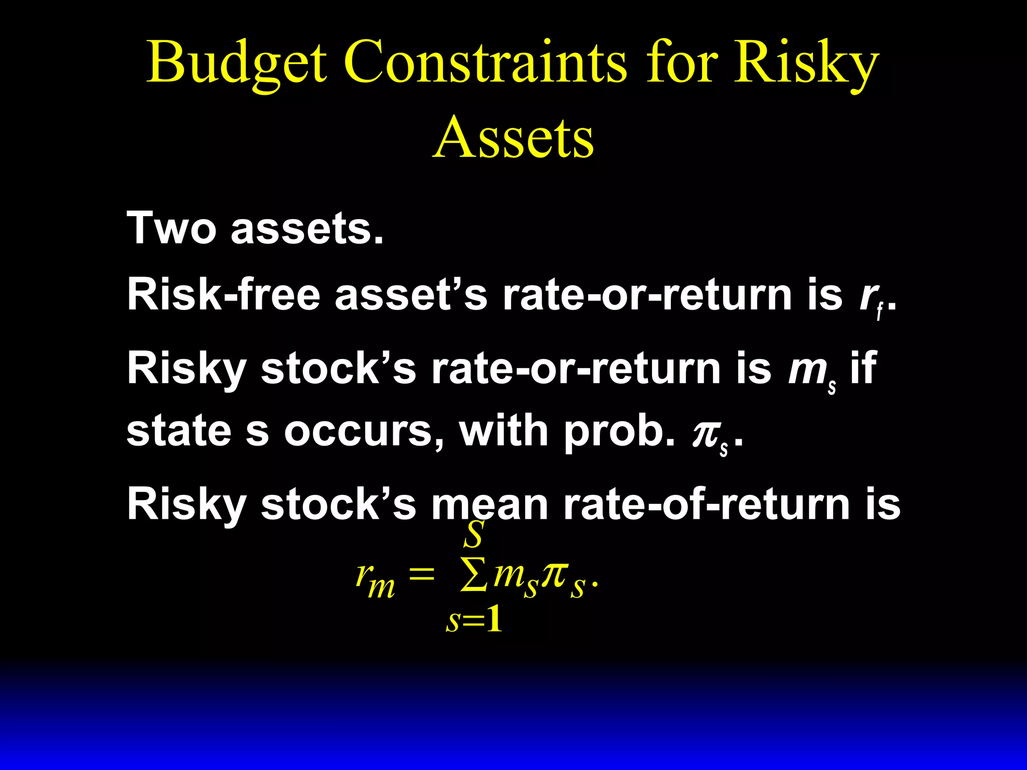
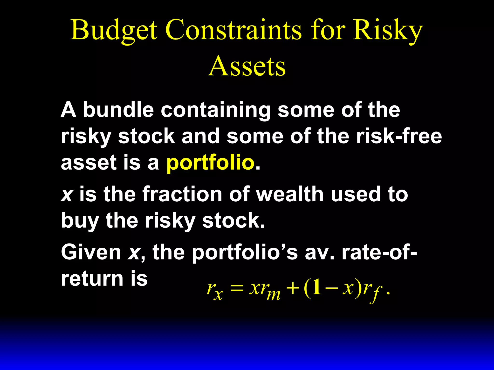
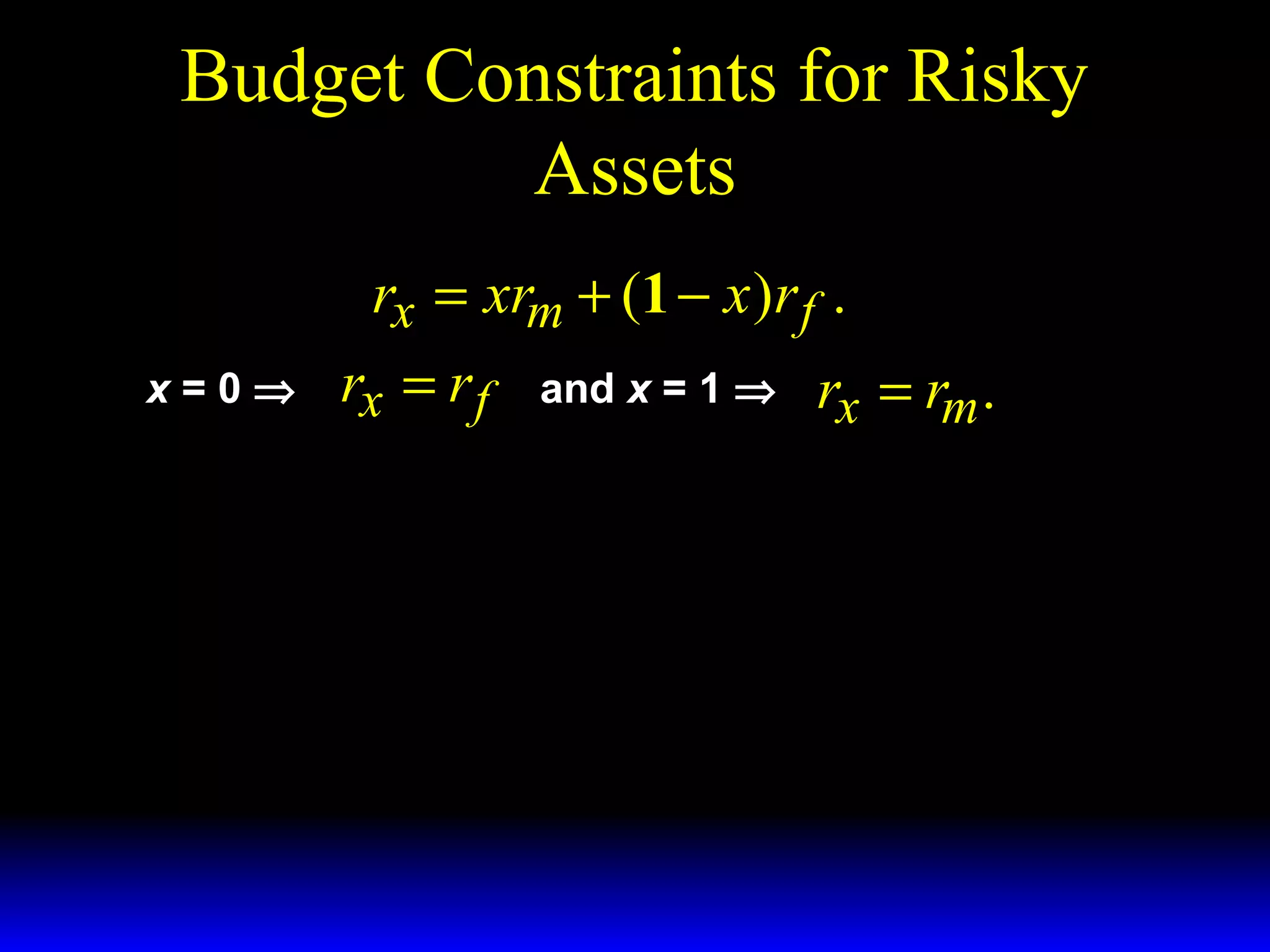
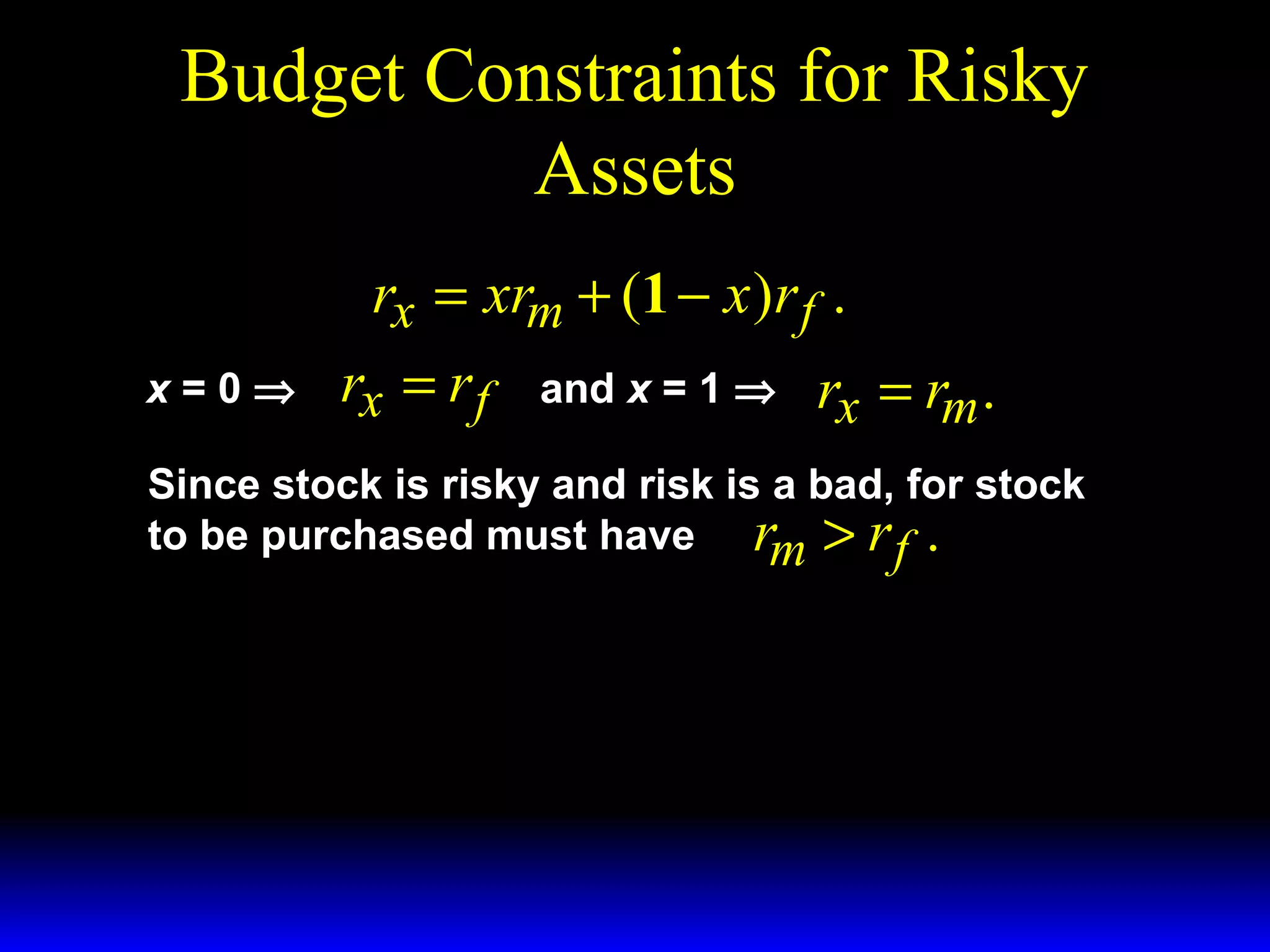
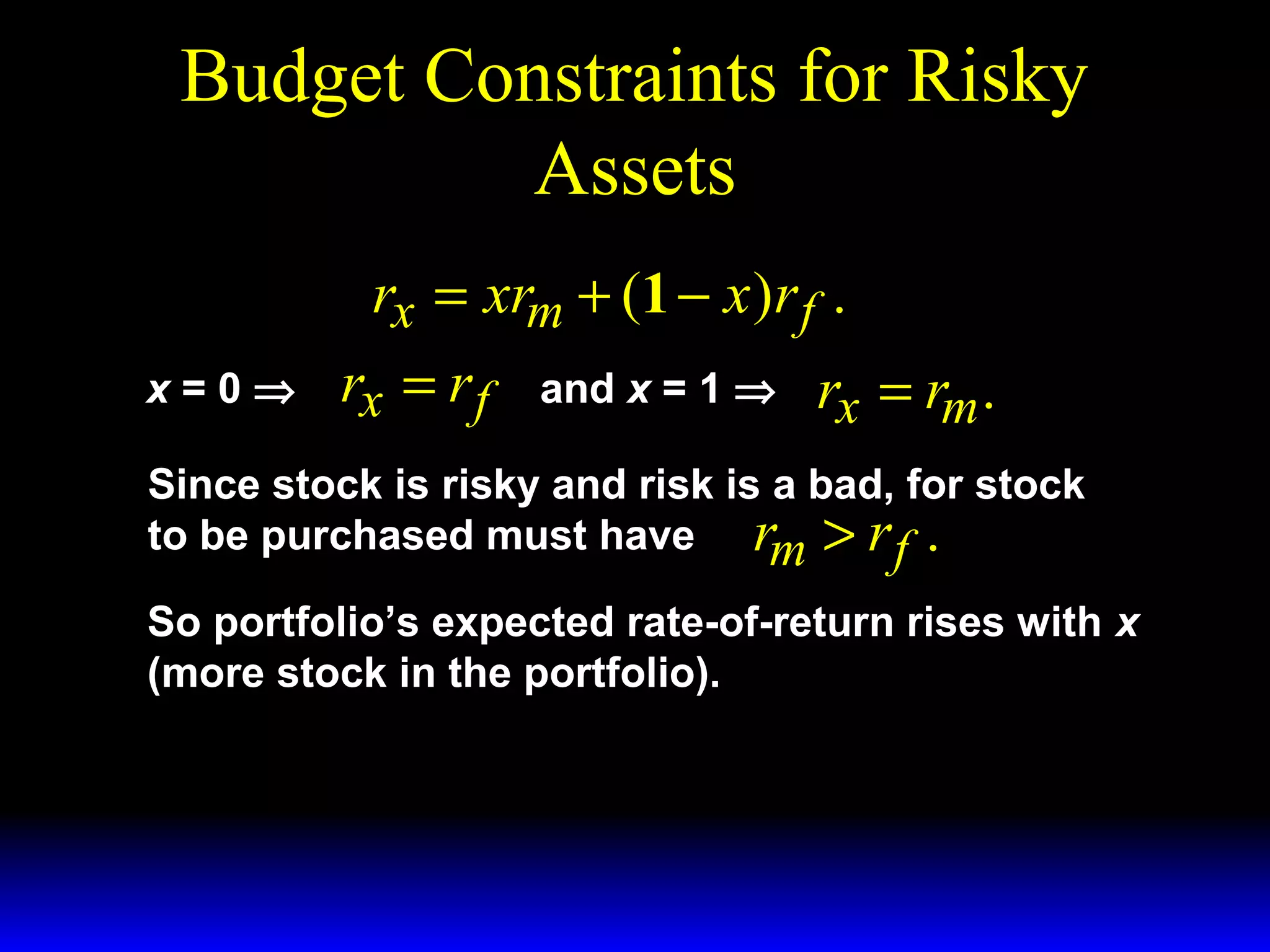
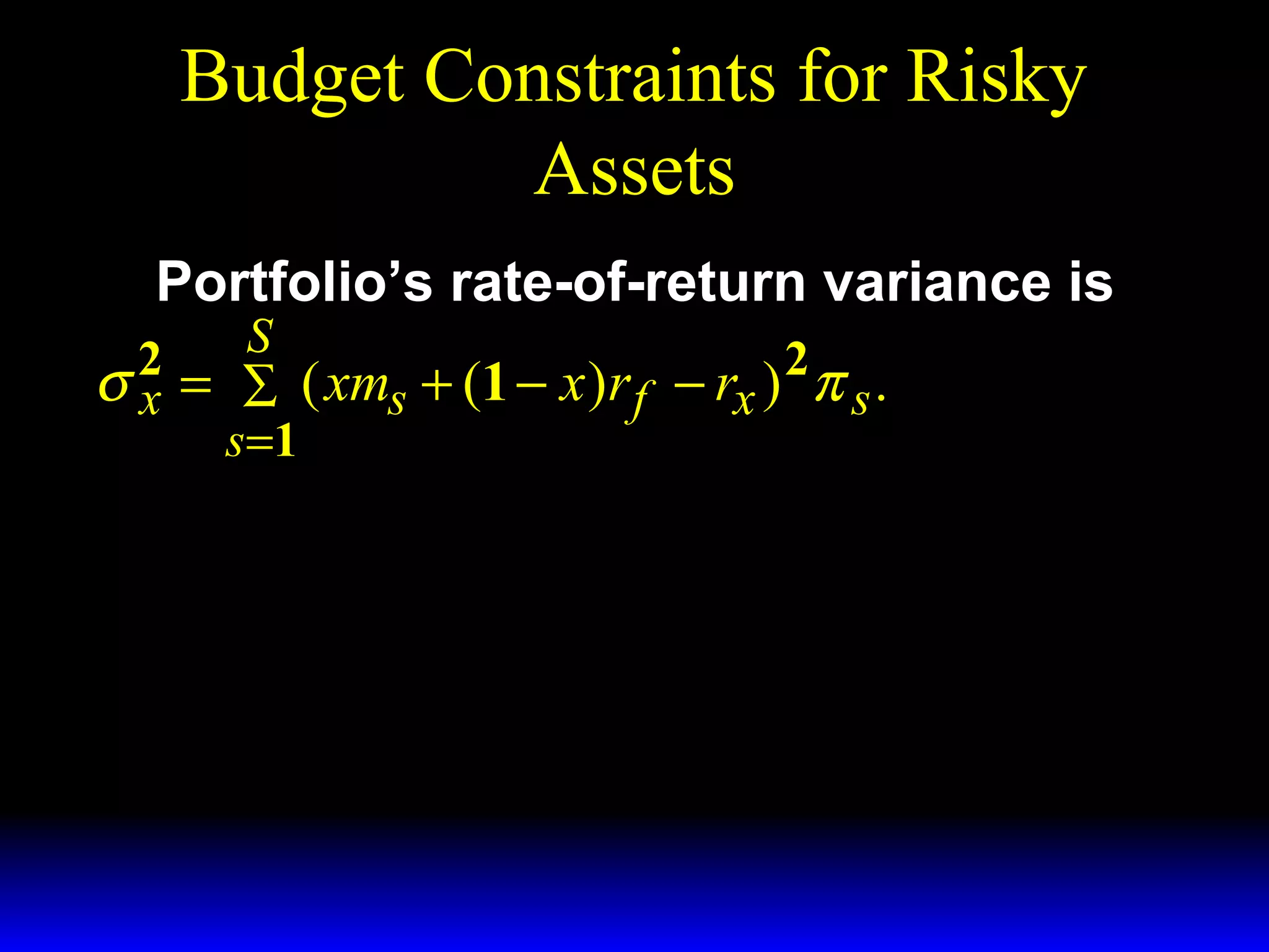
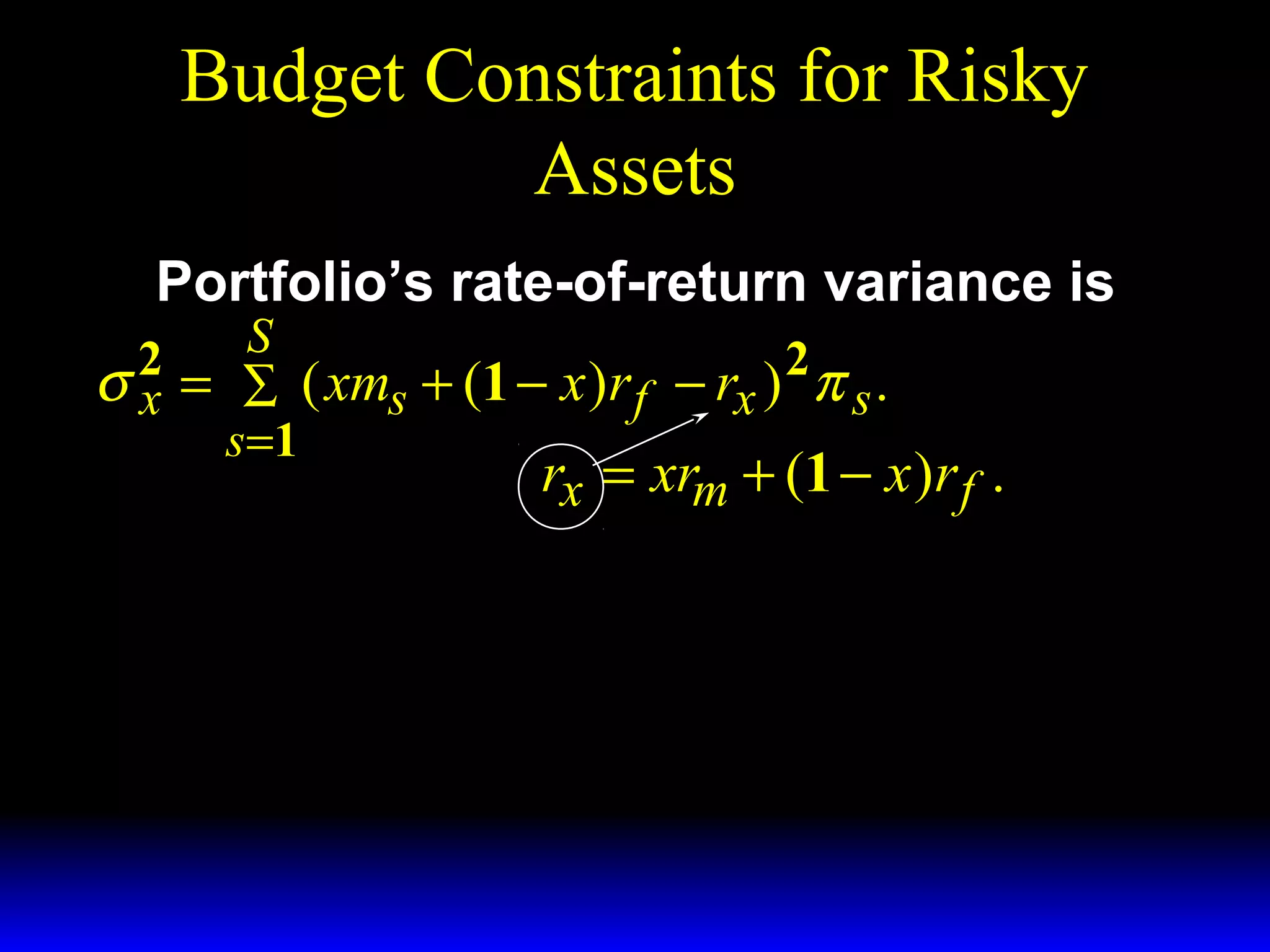
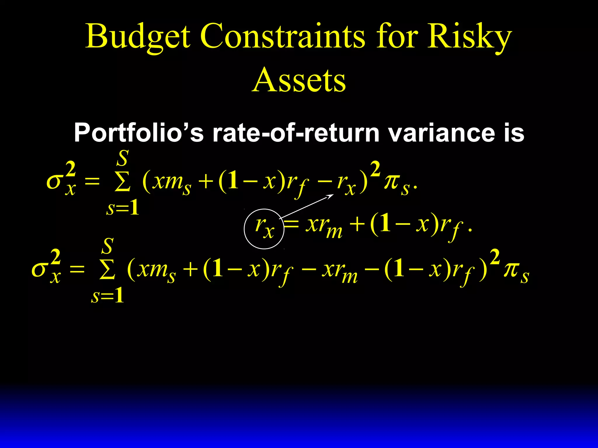
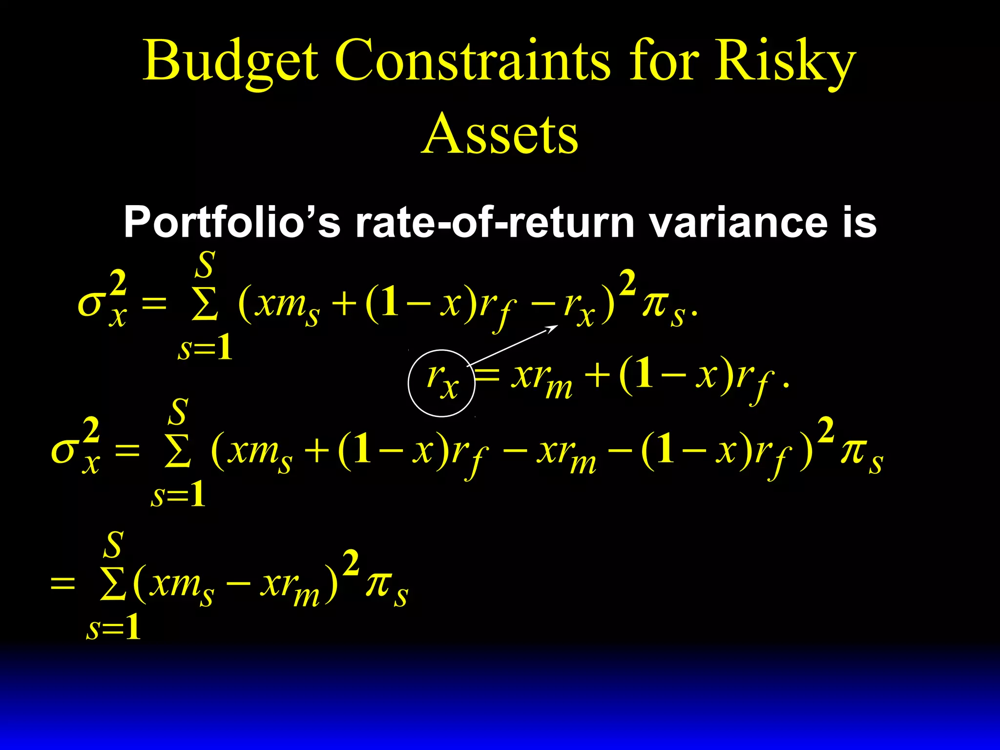
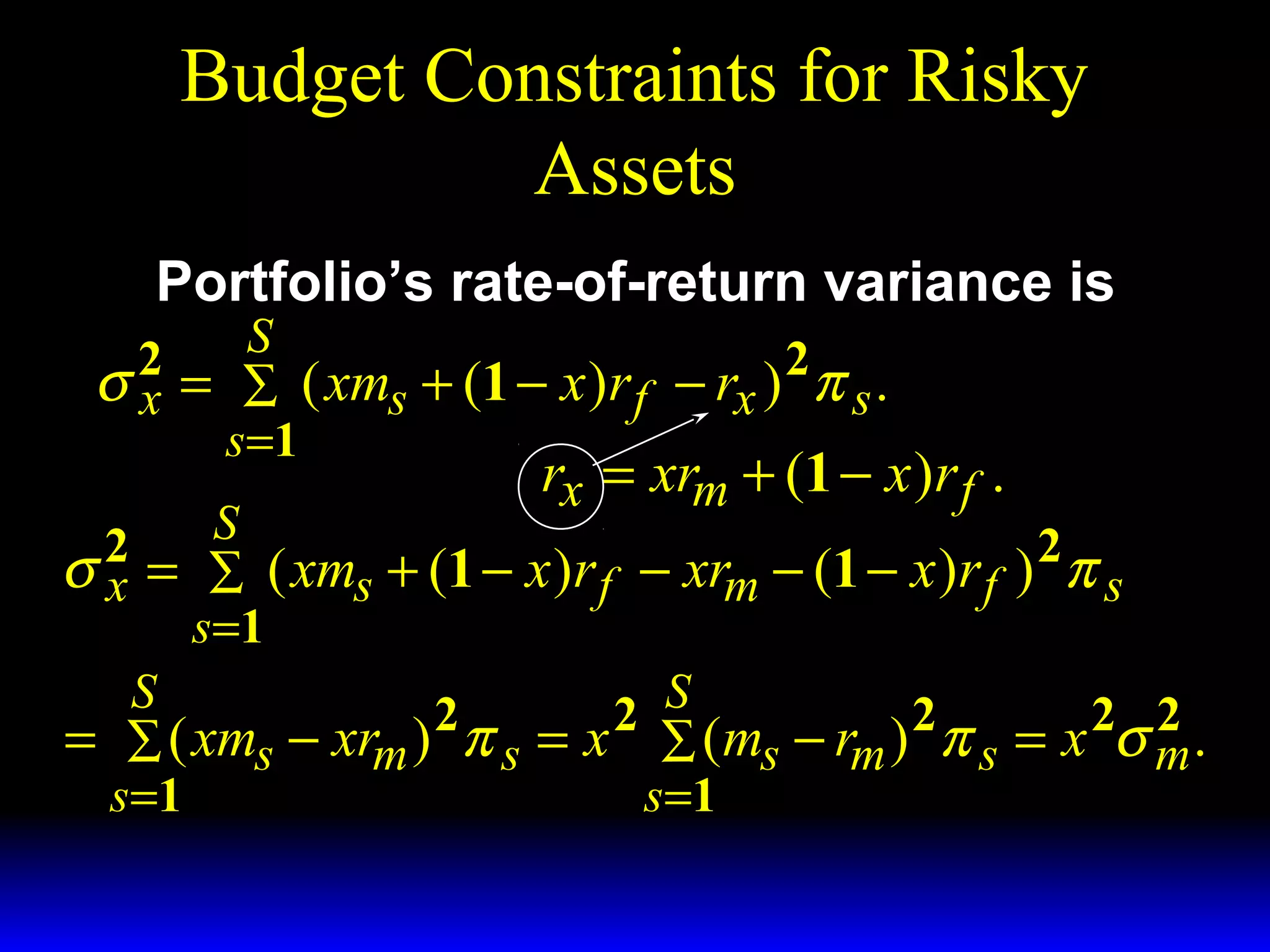
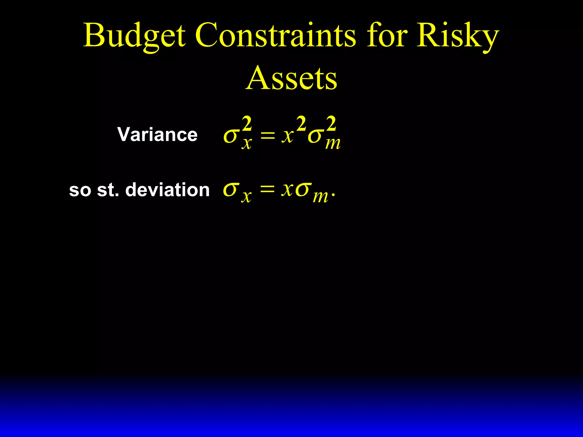
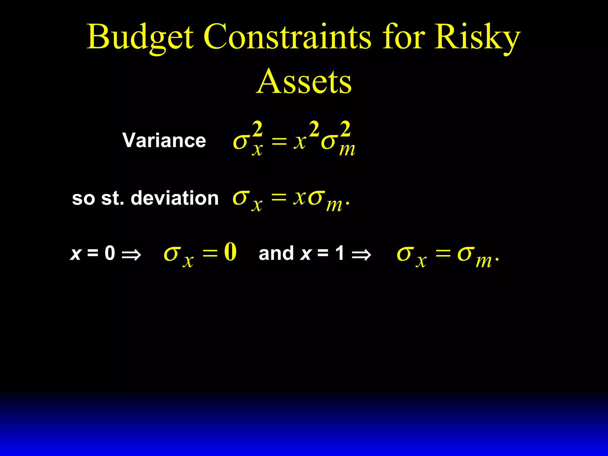
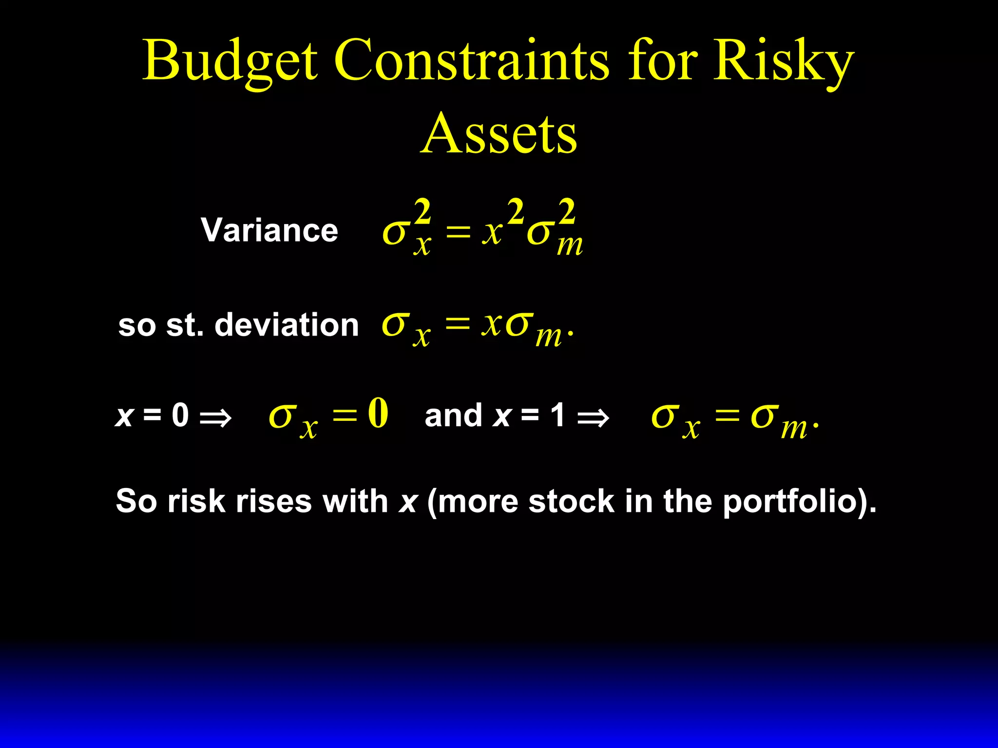
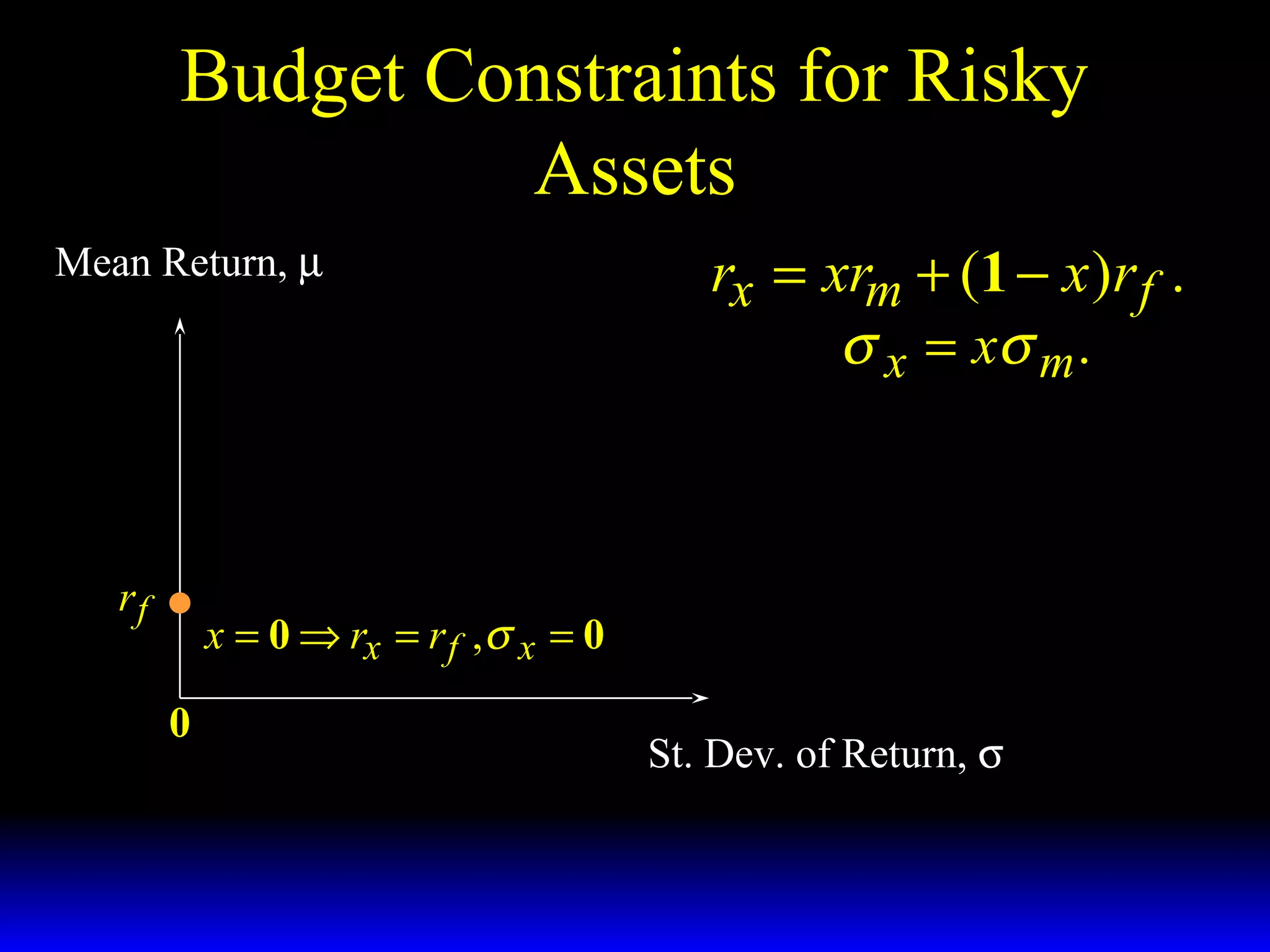
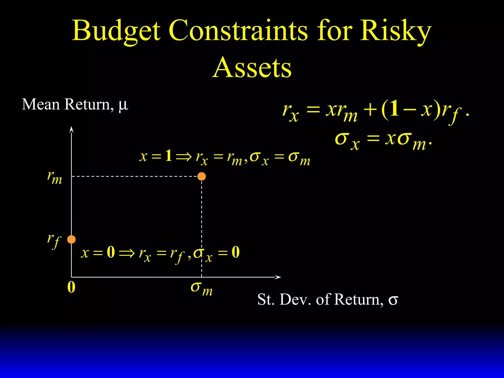
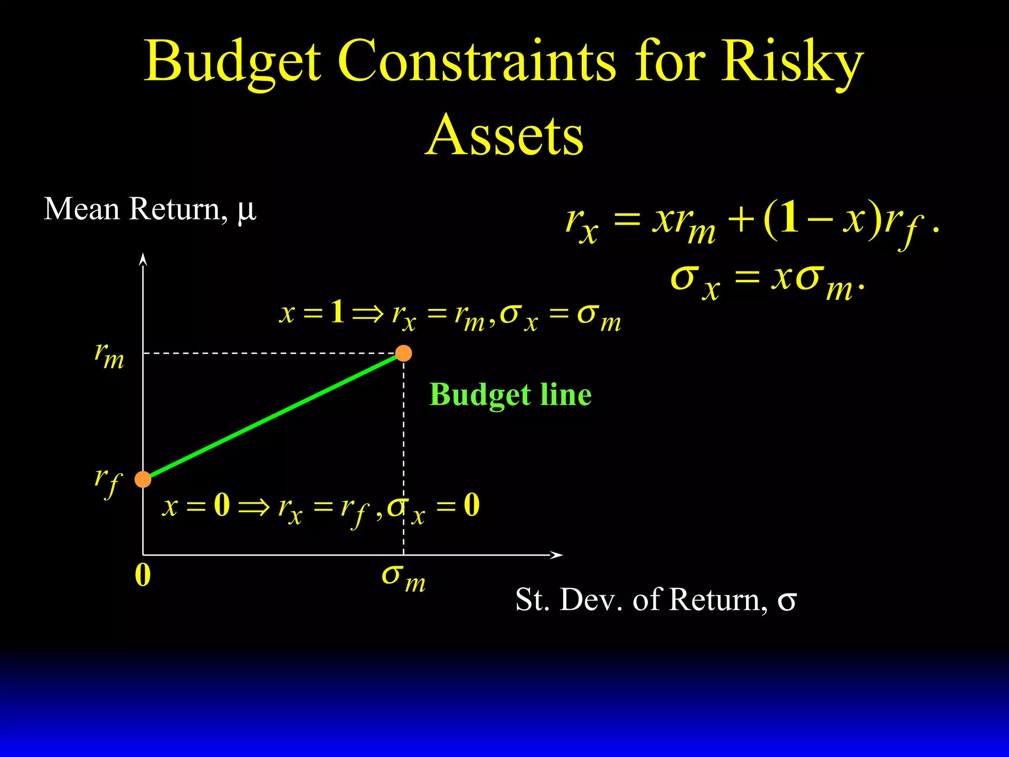
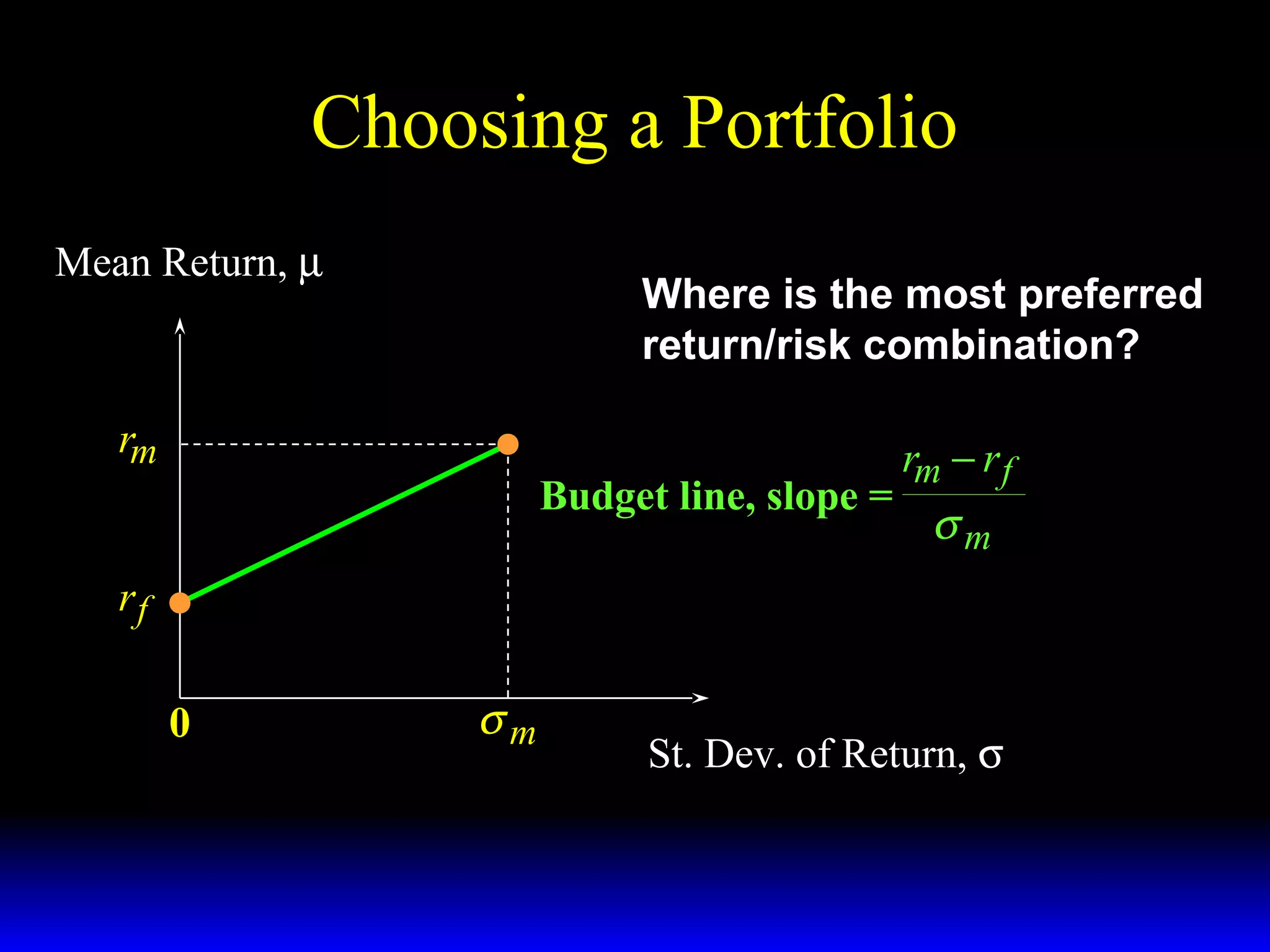
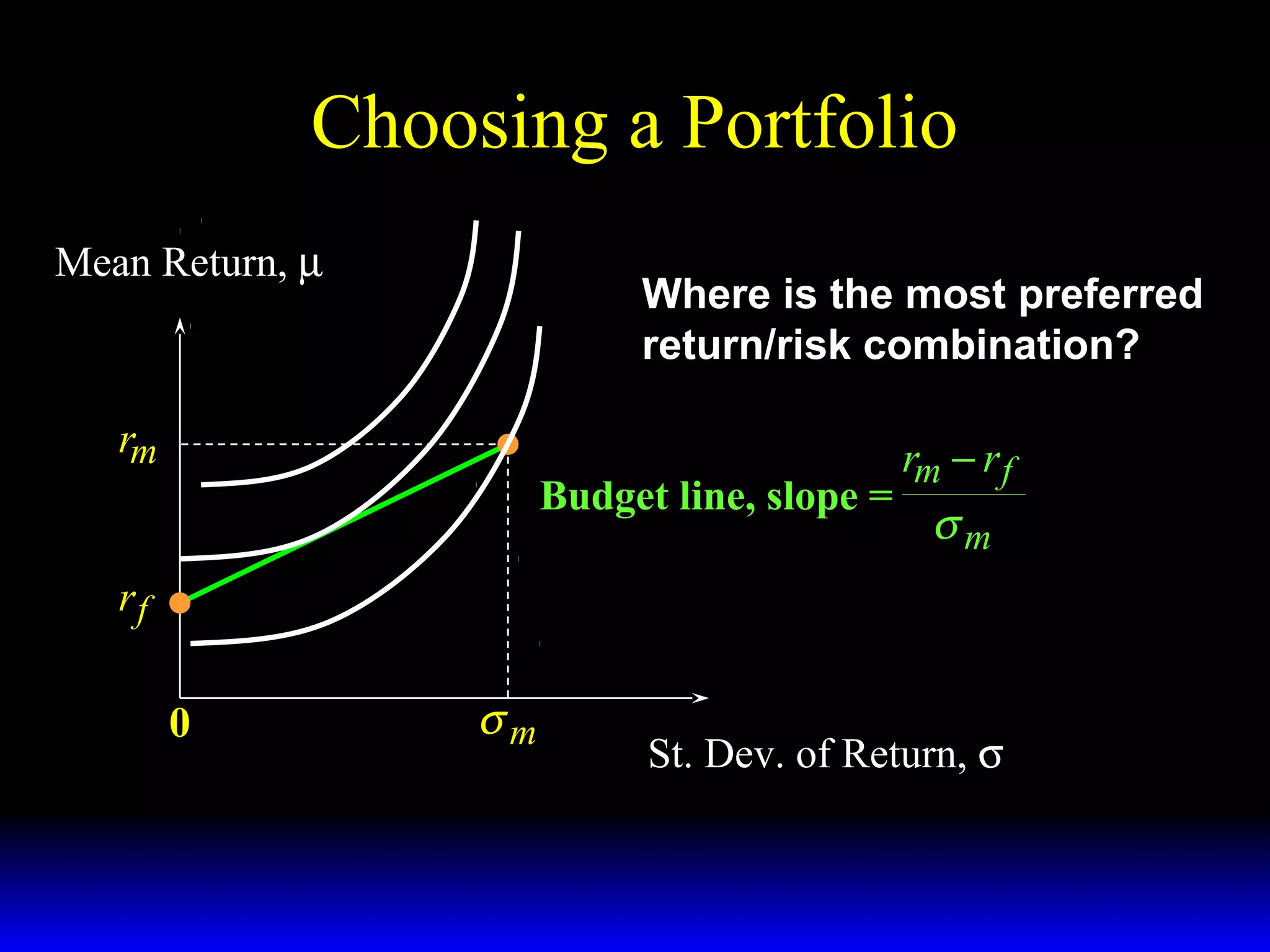
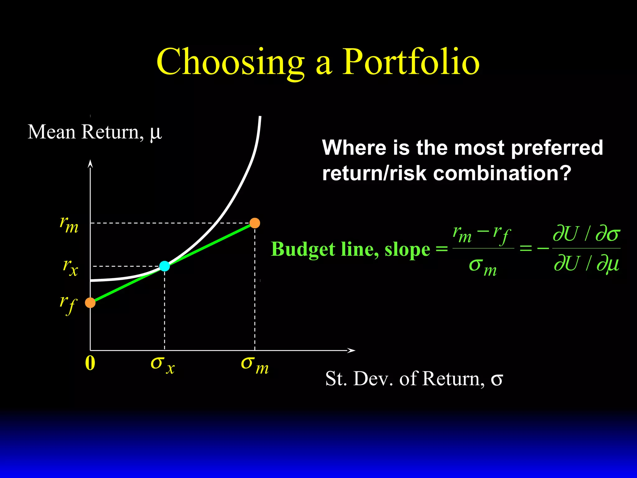
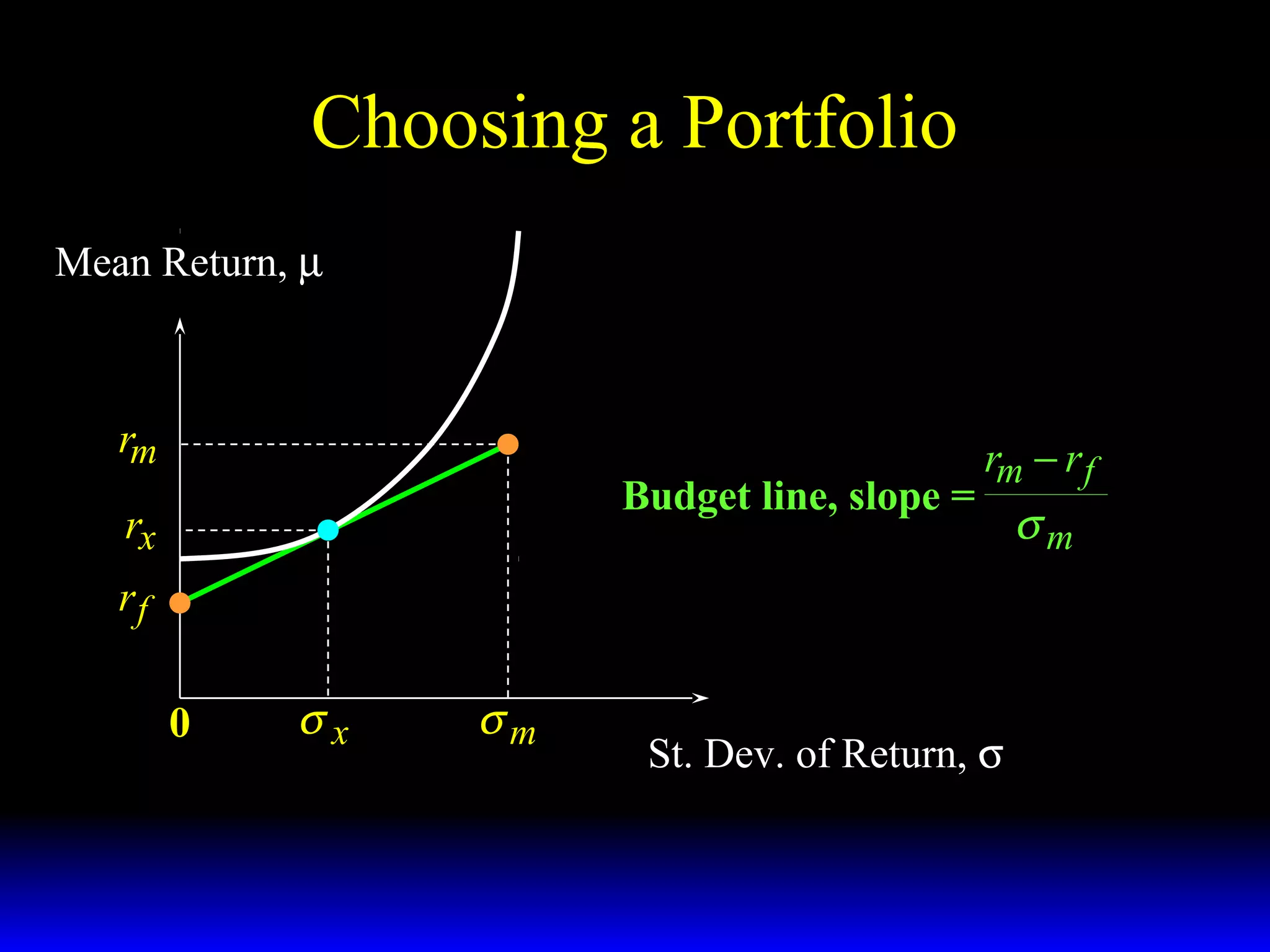
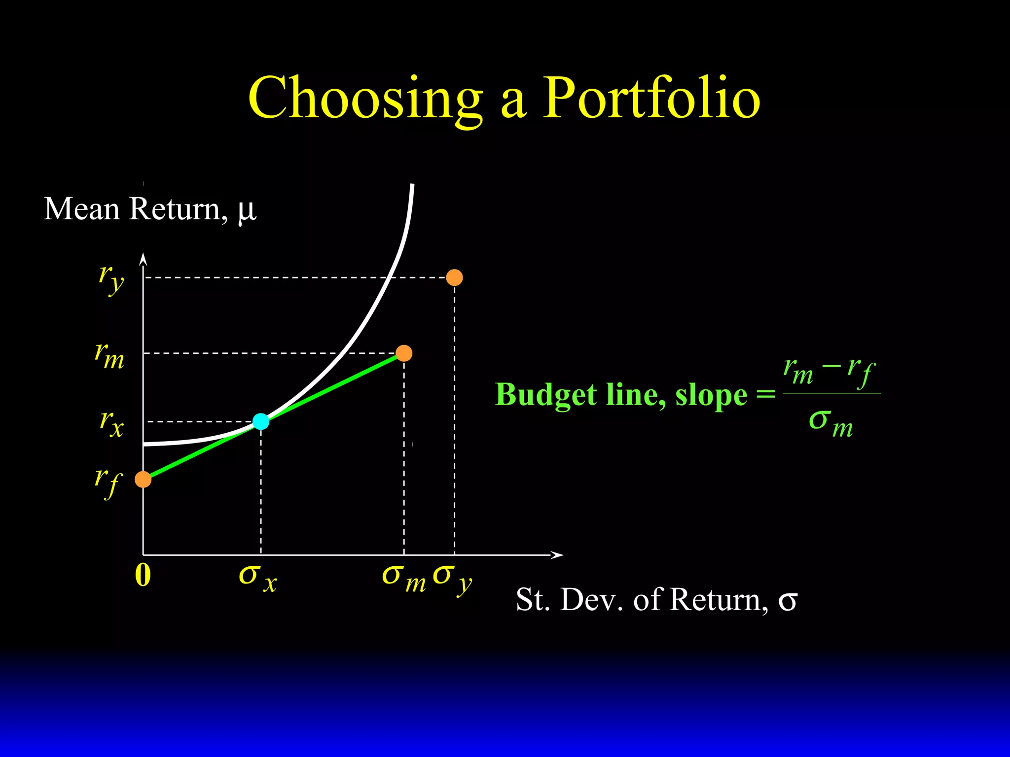
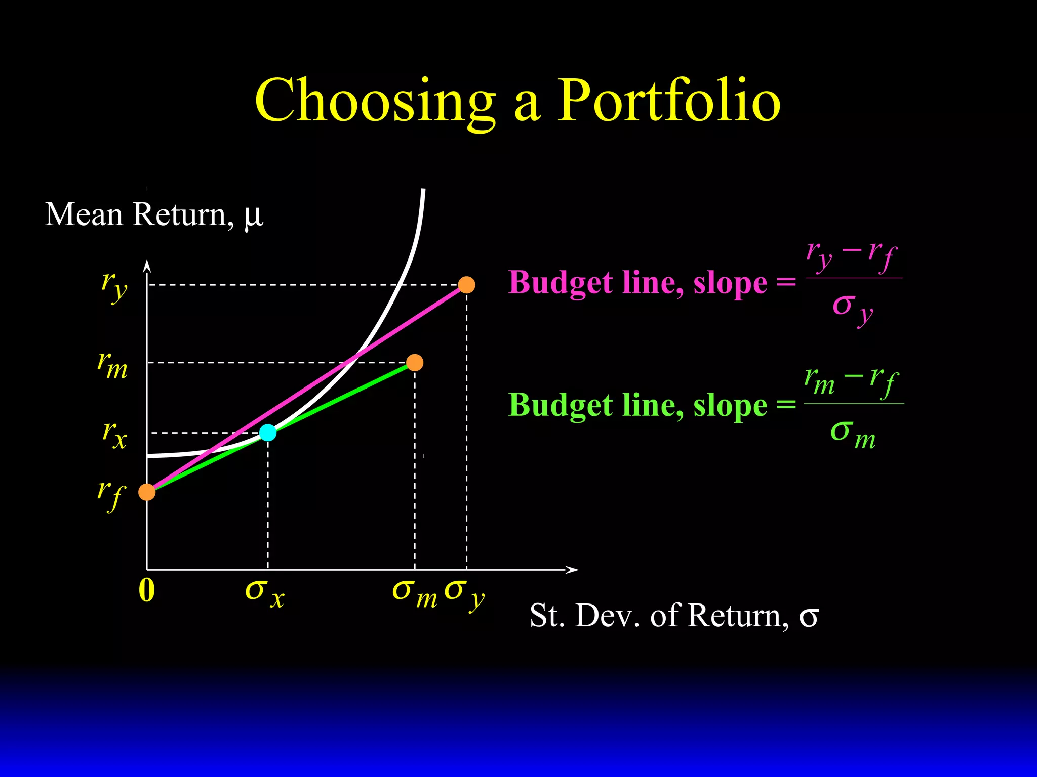
- The budget constraint for risky assets showing the tradeoff between expected return and risk of different portfolios.
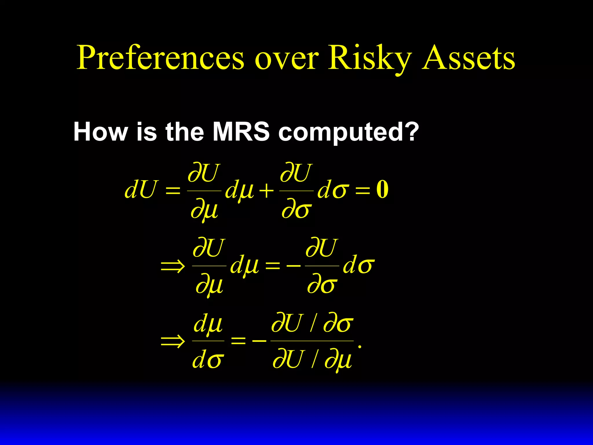
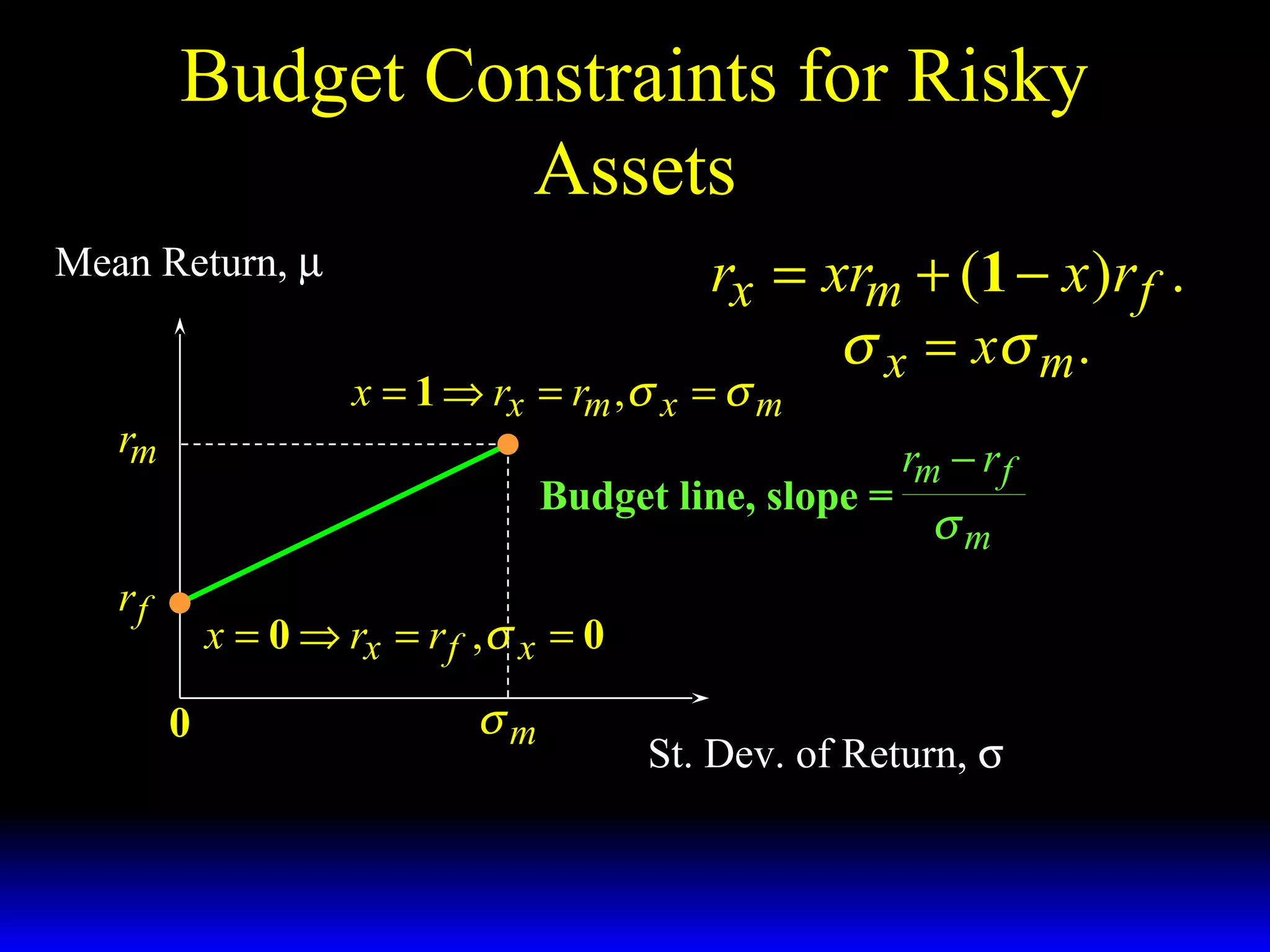
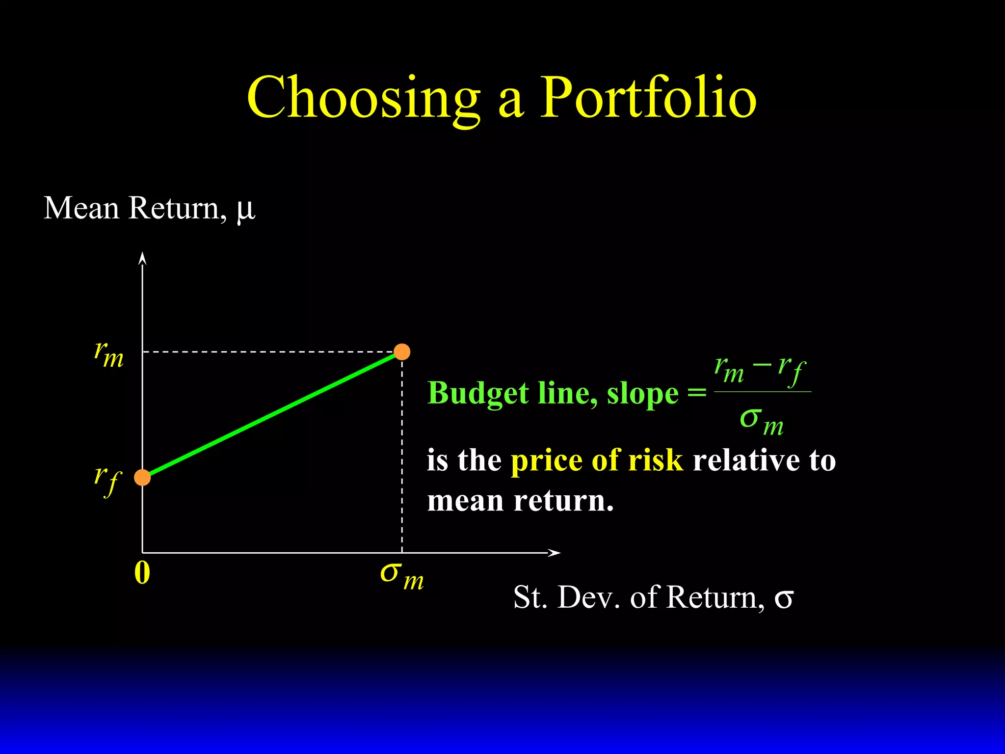
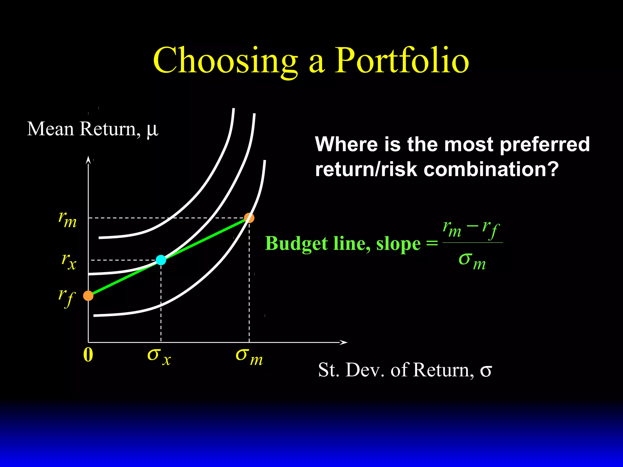
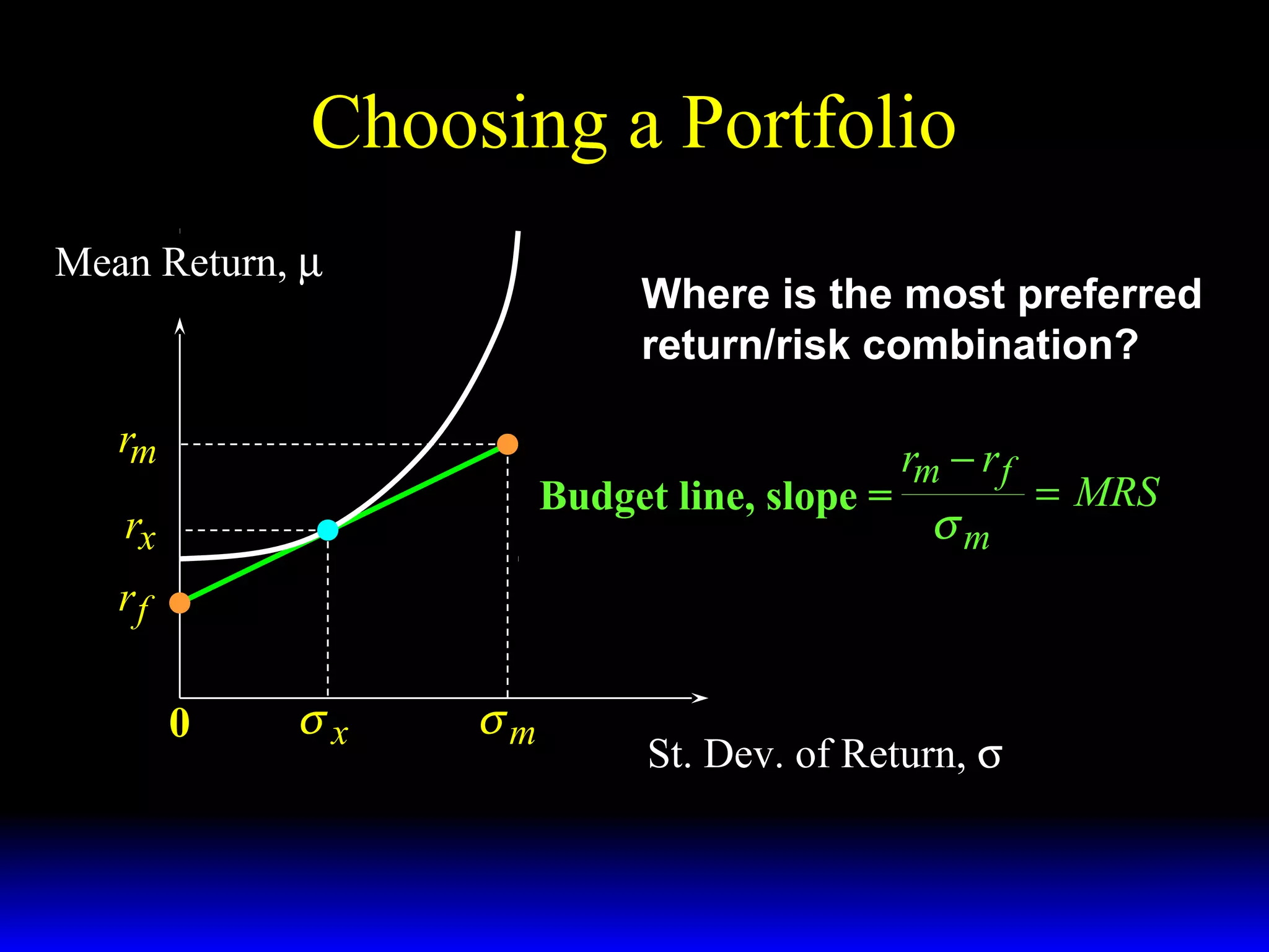
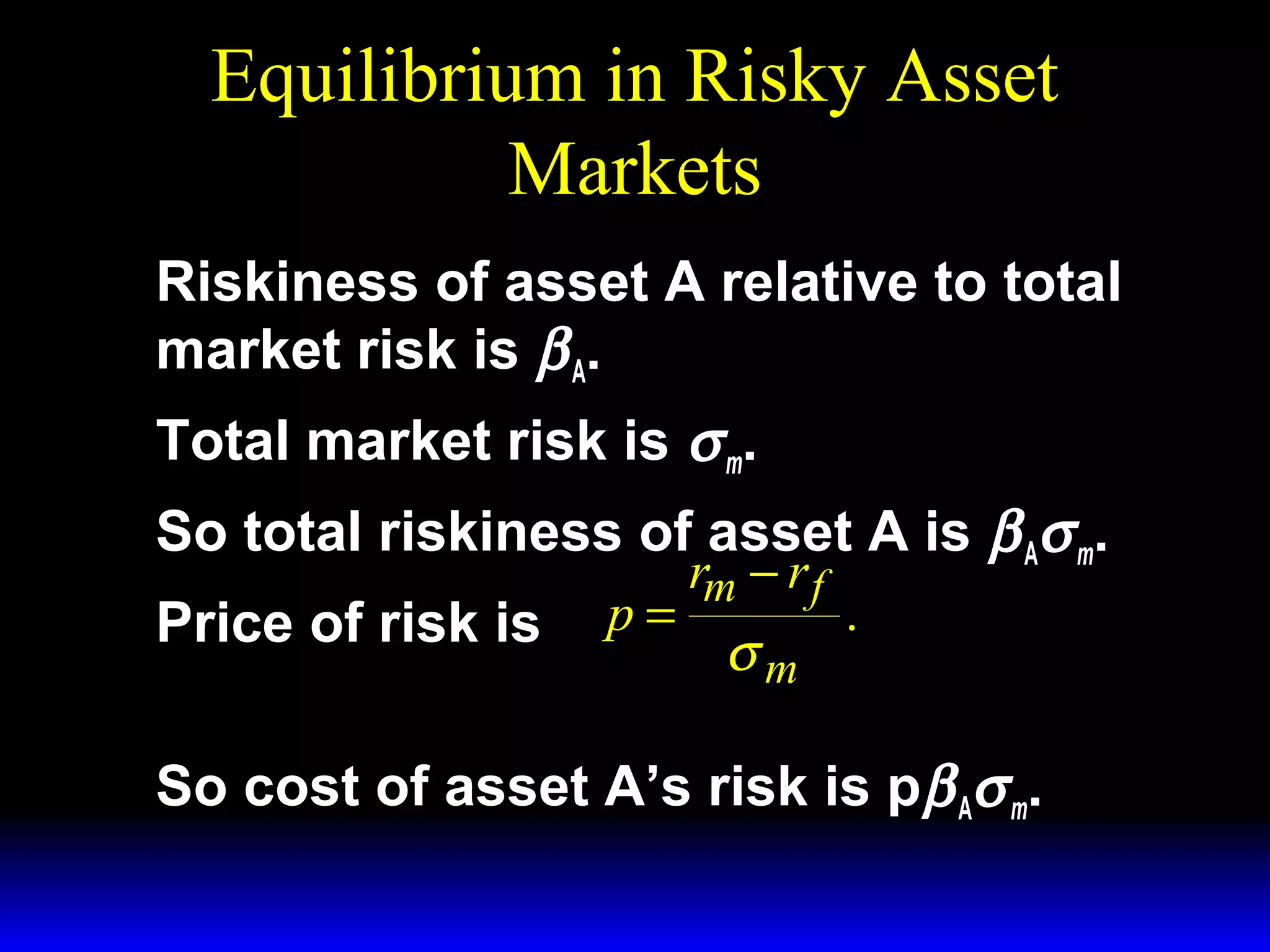
- How the slope of the budget constraint line represents the price of risk and most preferred portfolios lie along the line where the marginal rate of substitution equals this price.
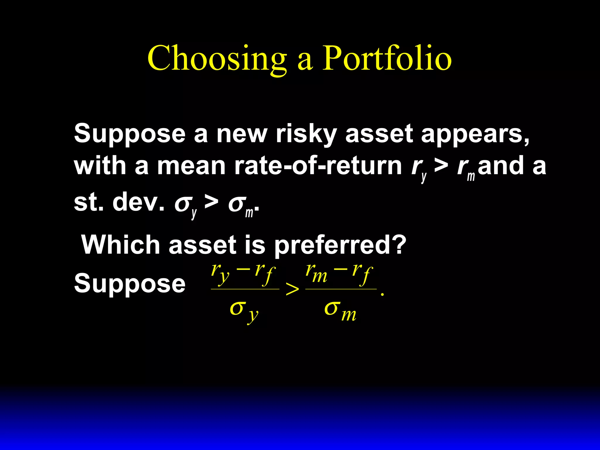
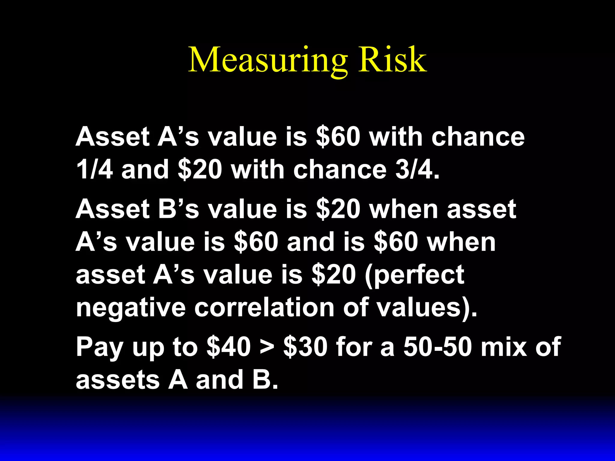
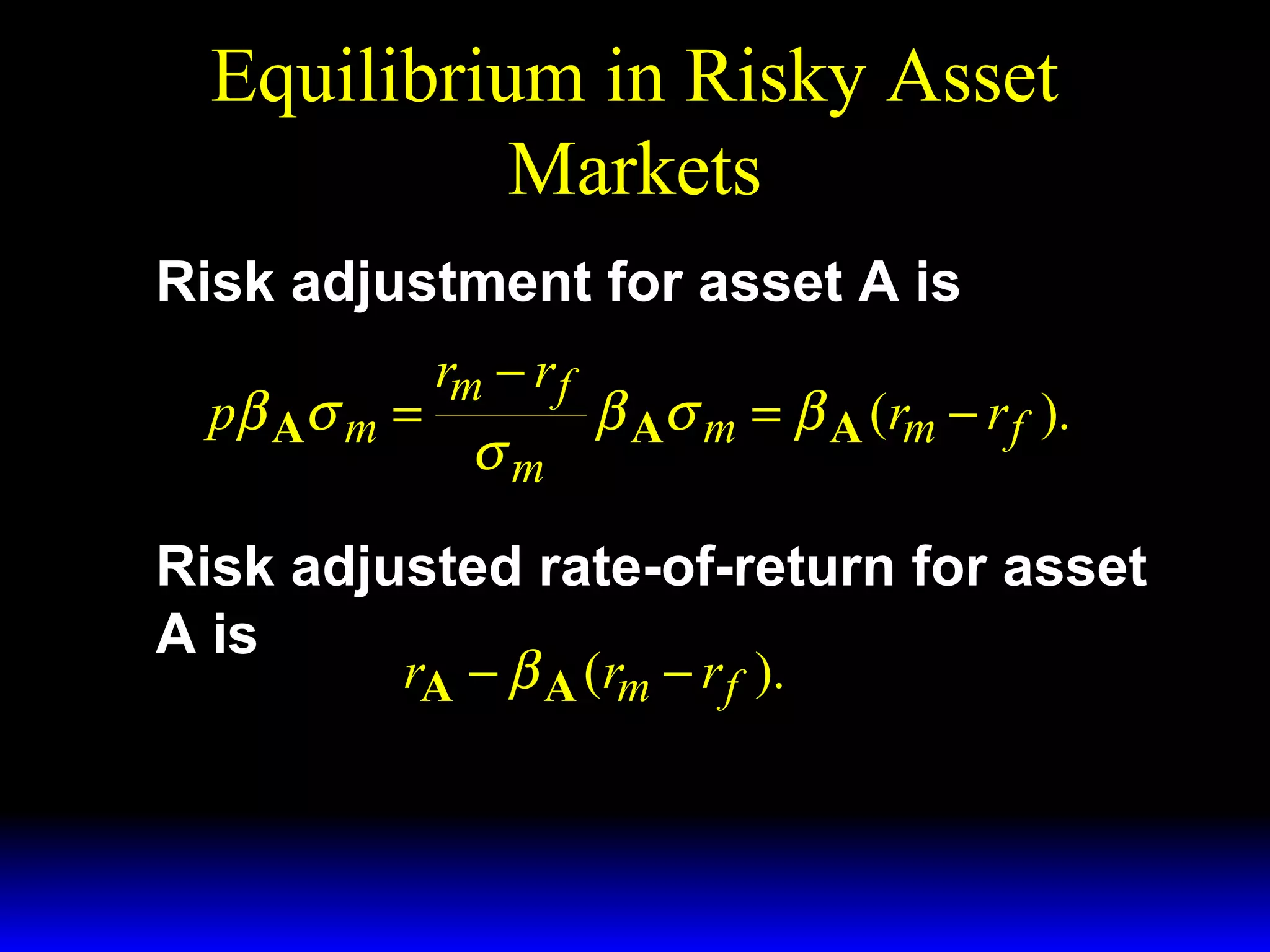
- Factors that influence choice between risky assets like their expected returns, risks, and risk-adjusted returns.
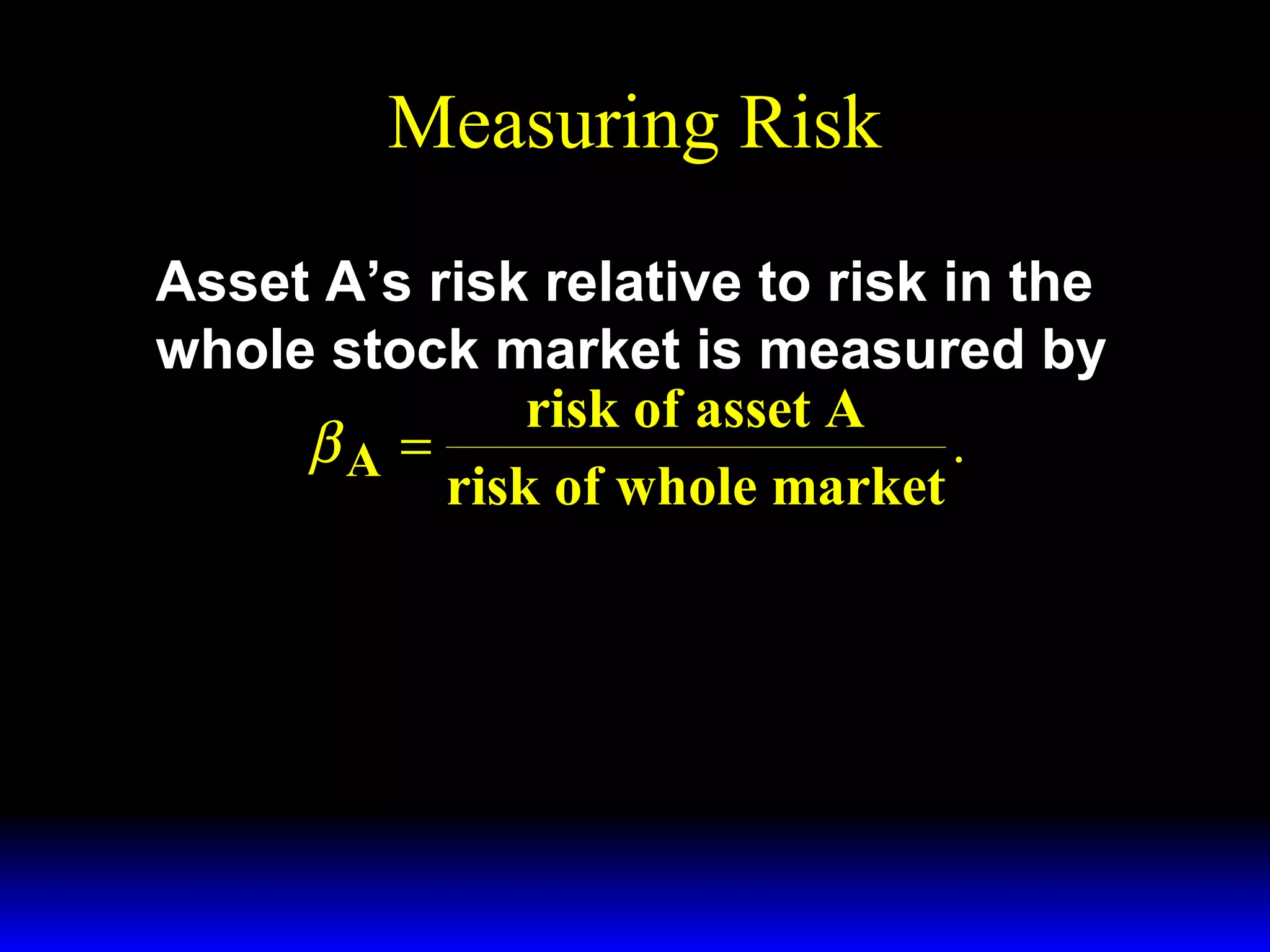
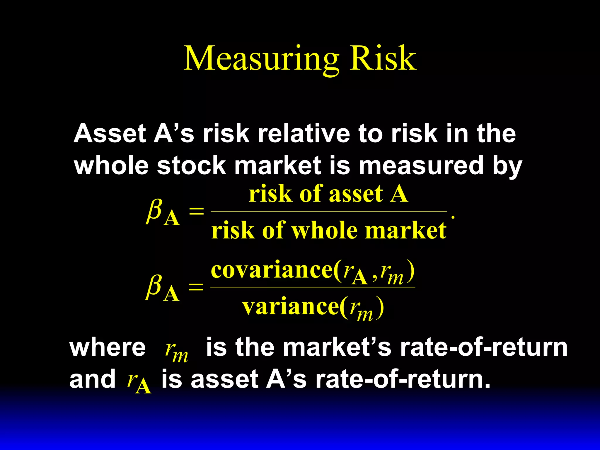
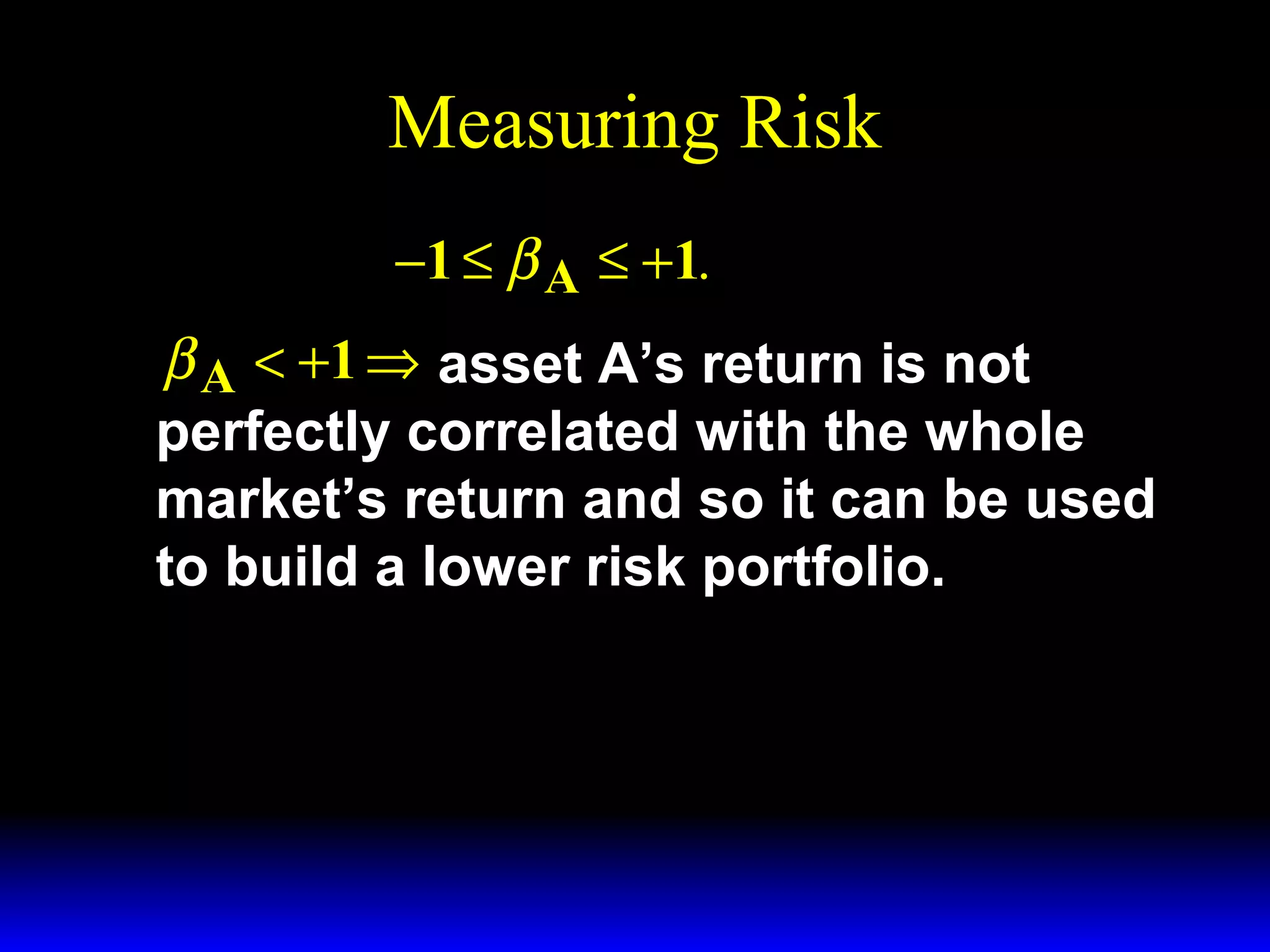
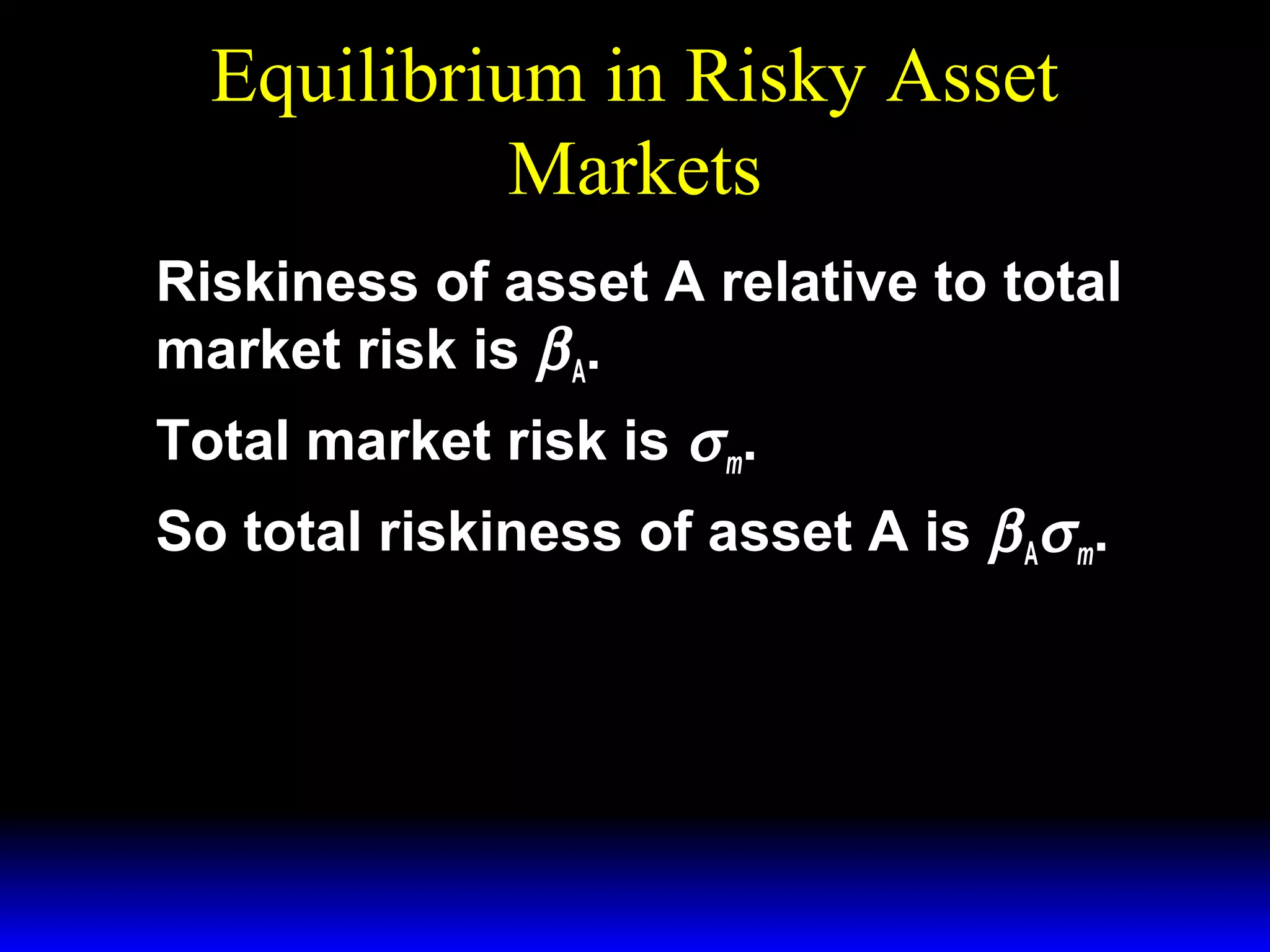
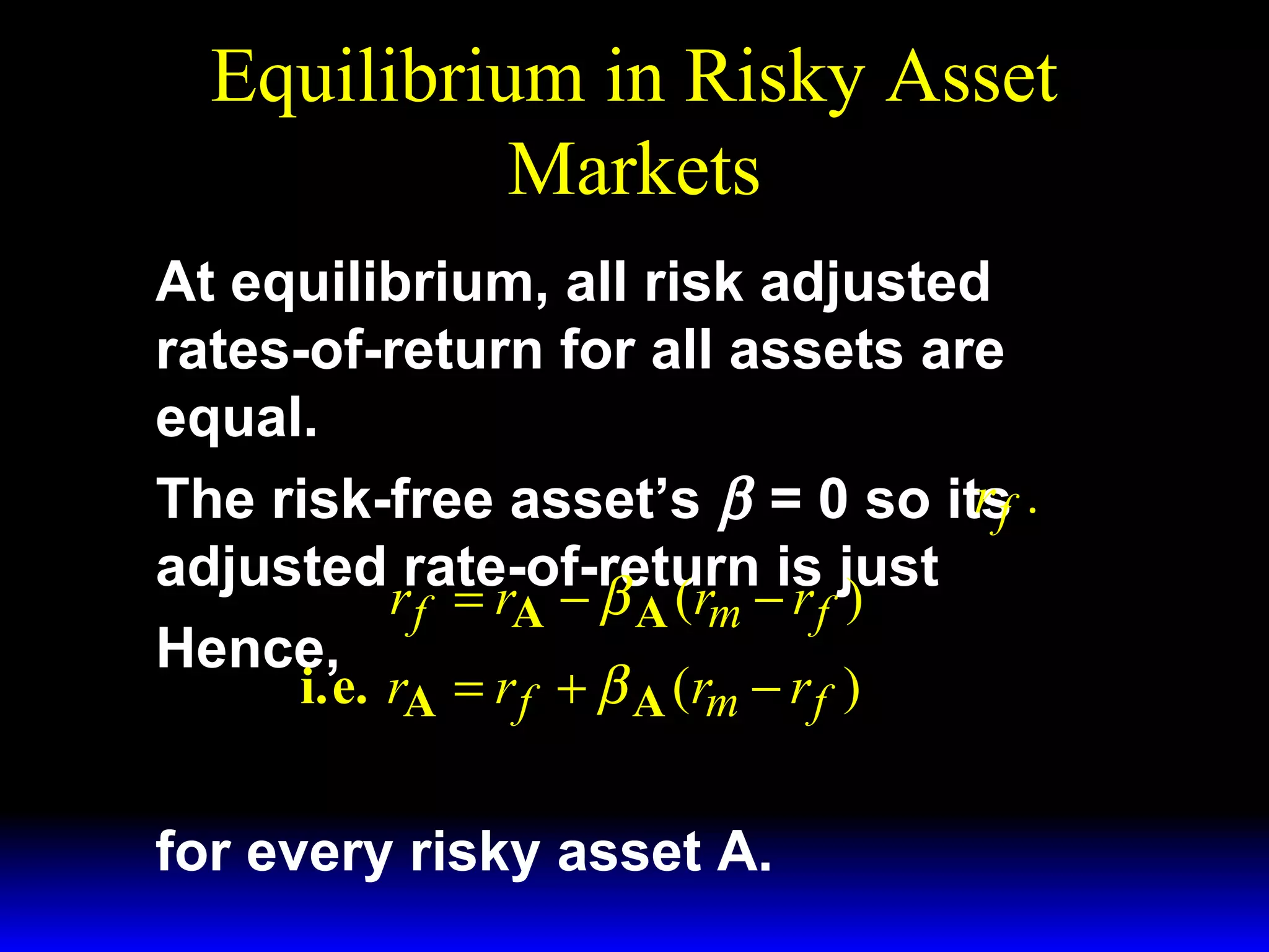
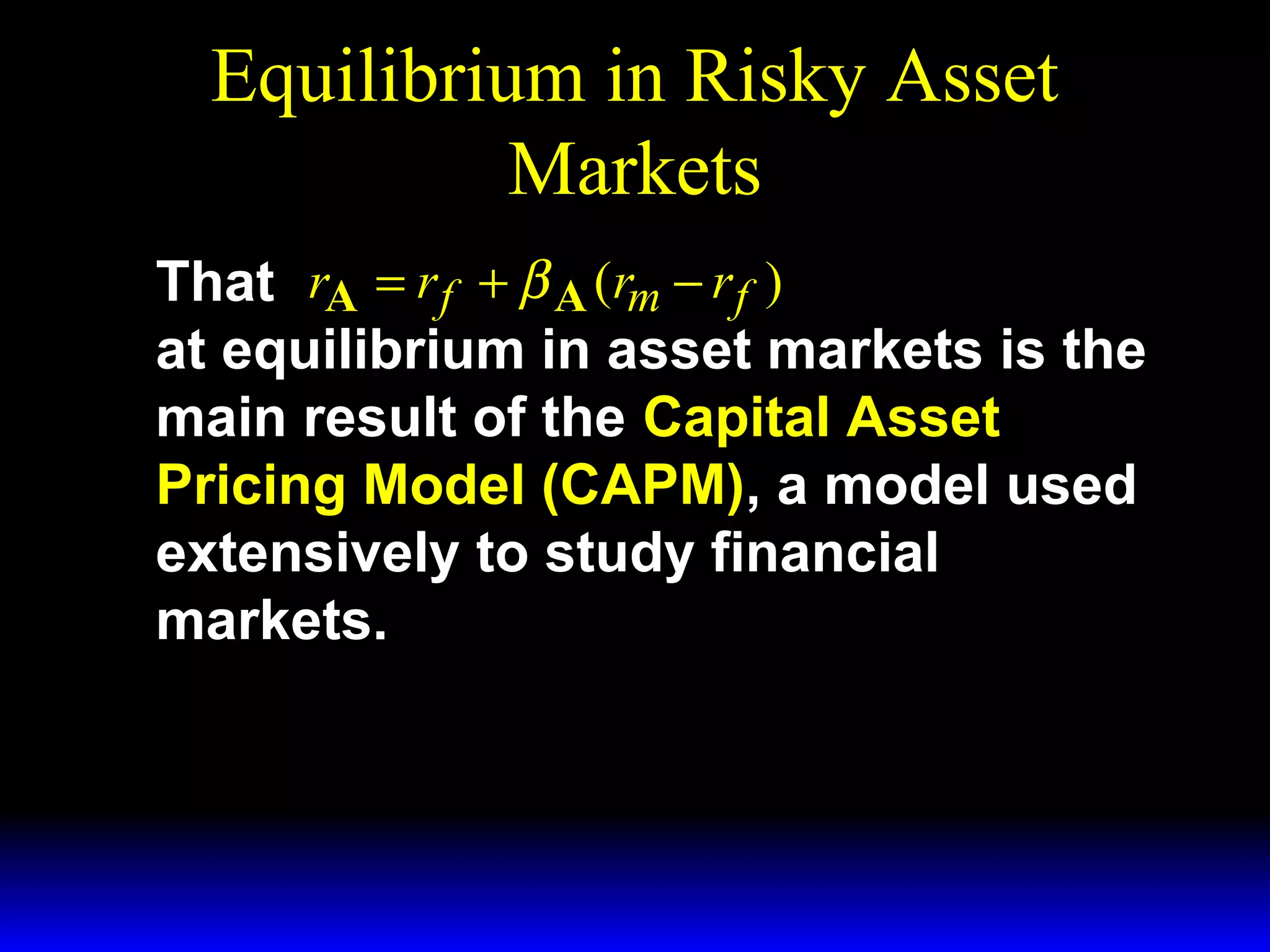
- Beta and how it measures the risk of individual
![Mean of a Distribution
A random variable (r.v.) w takes
values w1,…,wS with probabilities
π 1,...,π S (π 1 + · · · + π S = 1).
The mean (expected value) of the
distribution is the av. value of the
r.v.;
S
E[ w] = µ w = ∑ wsπ s .
s =1](https://image.slidesharecdn.com/ch13-140131134437-phpapp01/75/Ch13-2-2048.jpg)
![Variance of a Distribution
The distribution’s variance is the
r.v.’s av. squared deviation from the
mean;
S
2
2
var[ w] = σ w = ∑ ( ws − µ w ) π s .
s =1
Variance measures the r.v.’s
variation.](https://image.slidesharecdn.com/ch13-140131134437-phpapp01/75/Ch13-3-2048.jpg)
![Standard Deviation of a
Distribution
The distribution’s standard deviation
is the square root of its variance;
2
st. dev[ w] = σ w = σ w =
S
2
∑ ( ws − µ w ) π s .
s =1
St. deviation also measures the r.v.’s
variability.](https://image.slidesharecdn.com/ch13-140131134437-phpapp01/75/Ch13-4-2048.jpg)


![[EM-Sofyan] Monopoly and Monopsony Market](https://cdn.slidesharecdn.com/ss_thumbnails/em-sofyanmonopolyandmonopsonymarket-140107174254-phpapp02-thumbnail.jpg?width=640&height=640&fit=bounds)