Downloaded 20 times


![Intermediate Macroeconomics
5. Permanent Income Hypothesis
• LCH Model
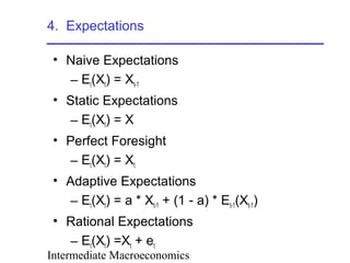
• Incorporates adaptive expectations to
explain how expectations of future income
are formed
• Current changes in income are considered
to be permanent based on:
YP = Y(t-1) + a [Y(t) - Y(t-1)]
• Consumption = c YP](https://image.slidesharecdn.com/ch10ppt-180115133341/85/Ch10ppt-18-320.jpg)


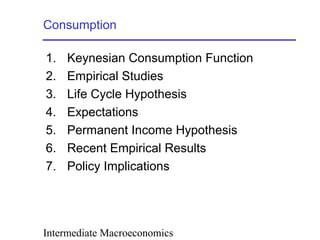
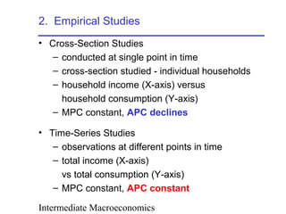
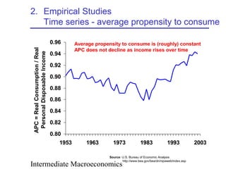
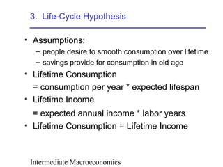
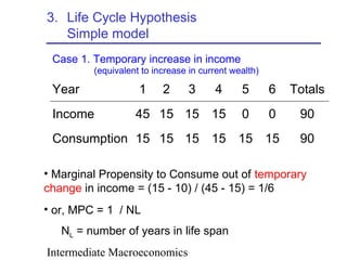
This document provides an overview of consumption and savings concepts covered in an intermediate macroeconomics textbook chapter. It discusses the Keynesian consumption function, empirical studies of consumption, the life cycle hypothesis of consumption, expectations theories, the permanent income hypothesis, and recent empirical work. Key models of consumption behavior are outlined, including how consumption responds to temporary versus permanent changes in income based on the life cycle hypothesis.