Downloaded 184 times
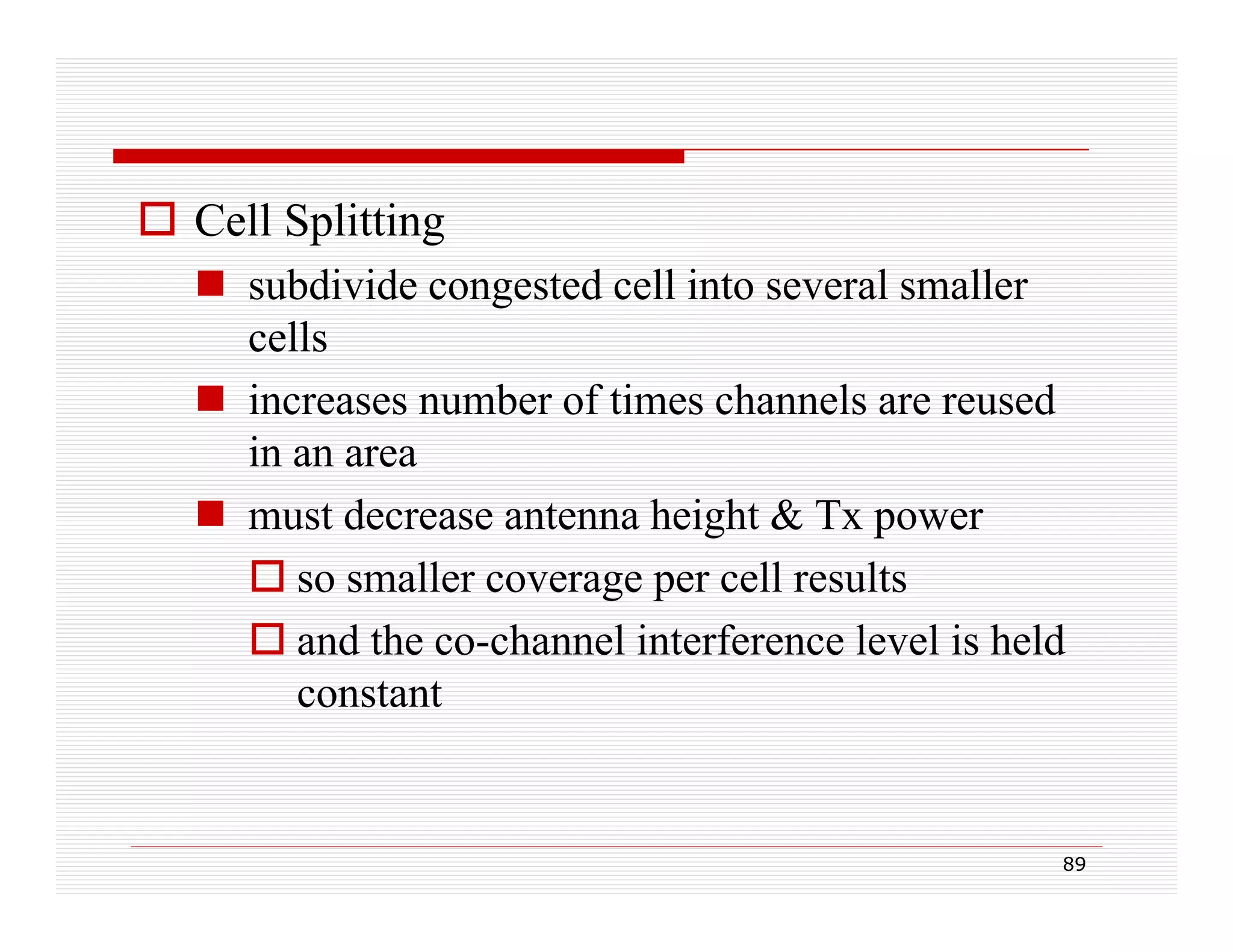
![ advantages include:
only needed for cells that reach max. capacity → not
all cells
implement when Pr [blocked call] > acceptable GOS
system capacity can gradually expand as demand ↑
disadvantages include:
# handoffs/unit area increases
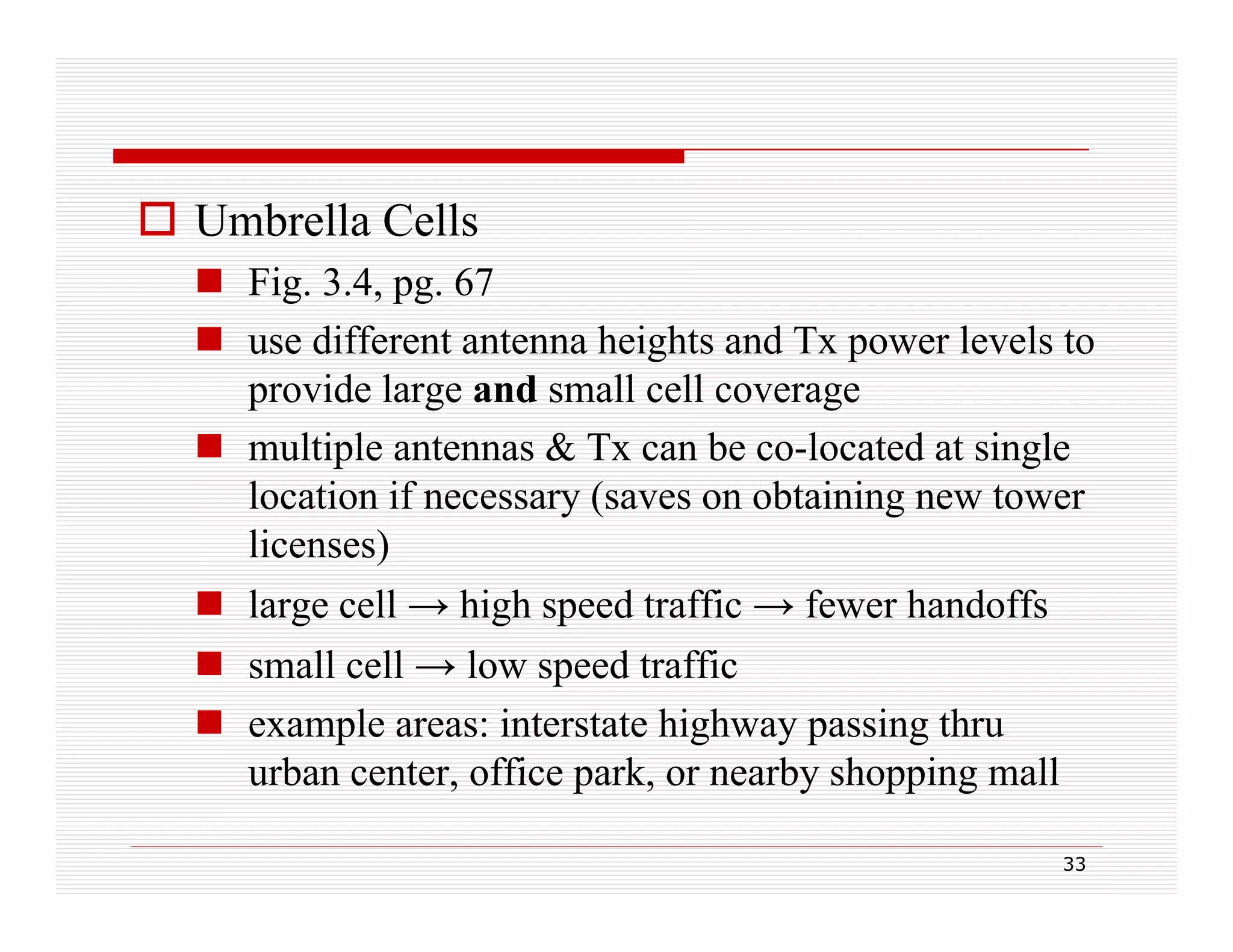
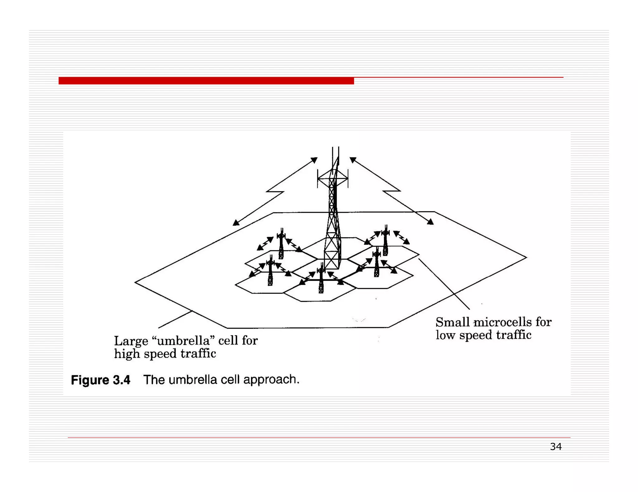
umbrella cell for high velocity traffic may be needed
more base stations → $$ for real estate, towers, etc.
92](https://image.slidesharecdn.com/cellularconcepts-131019201257-phpapp01/75/Cellular-concepts-92-2048.jpg)
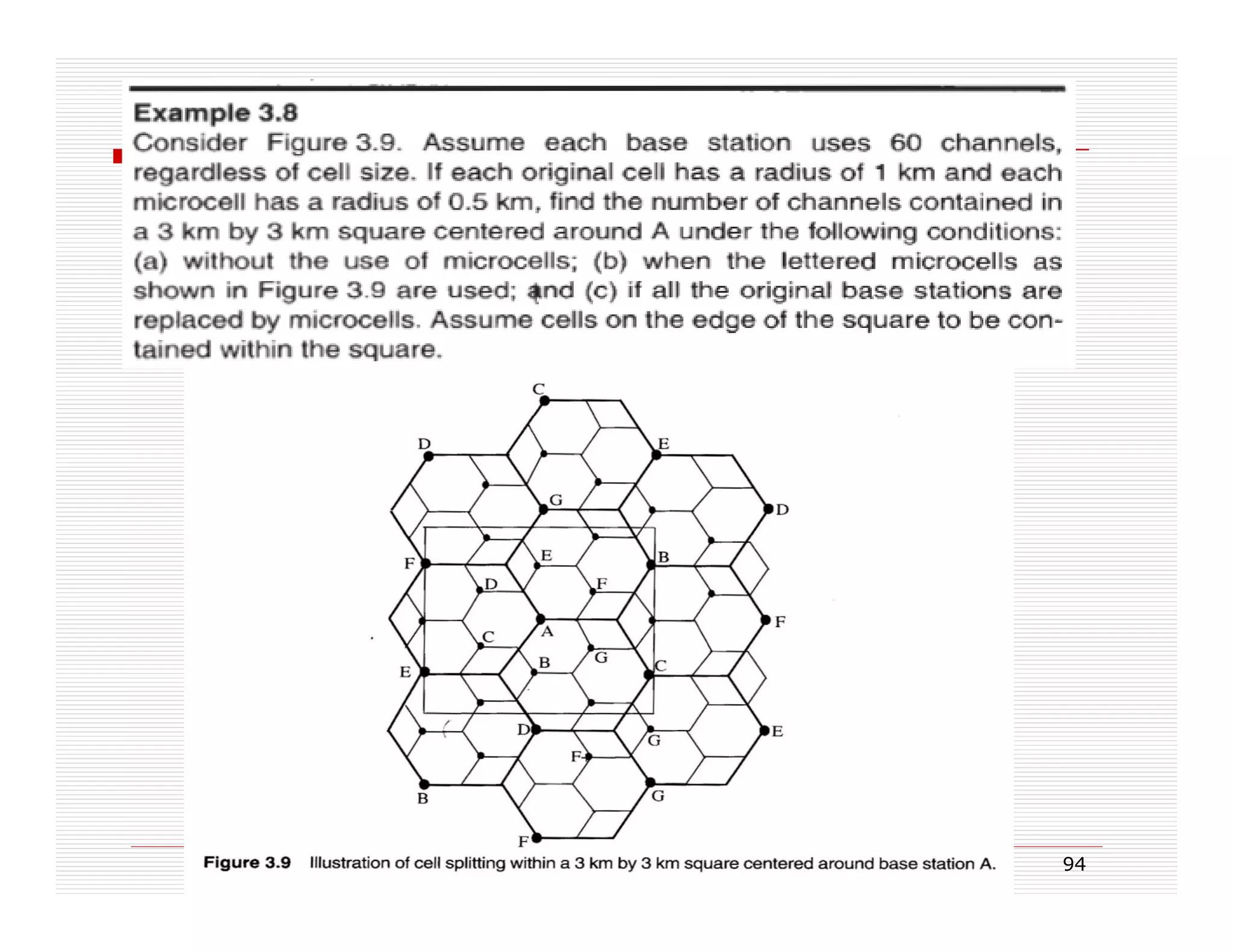

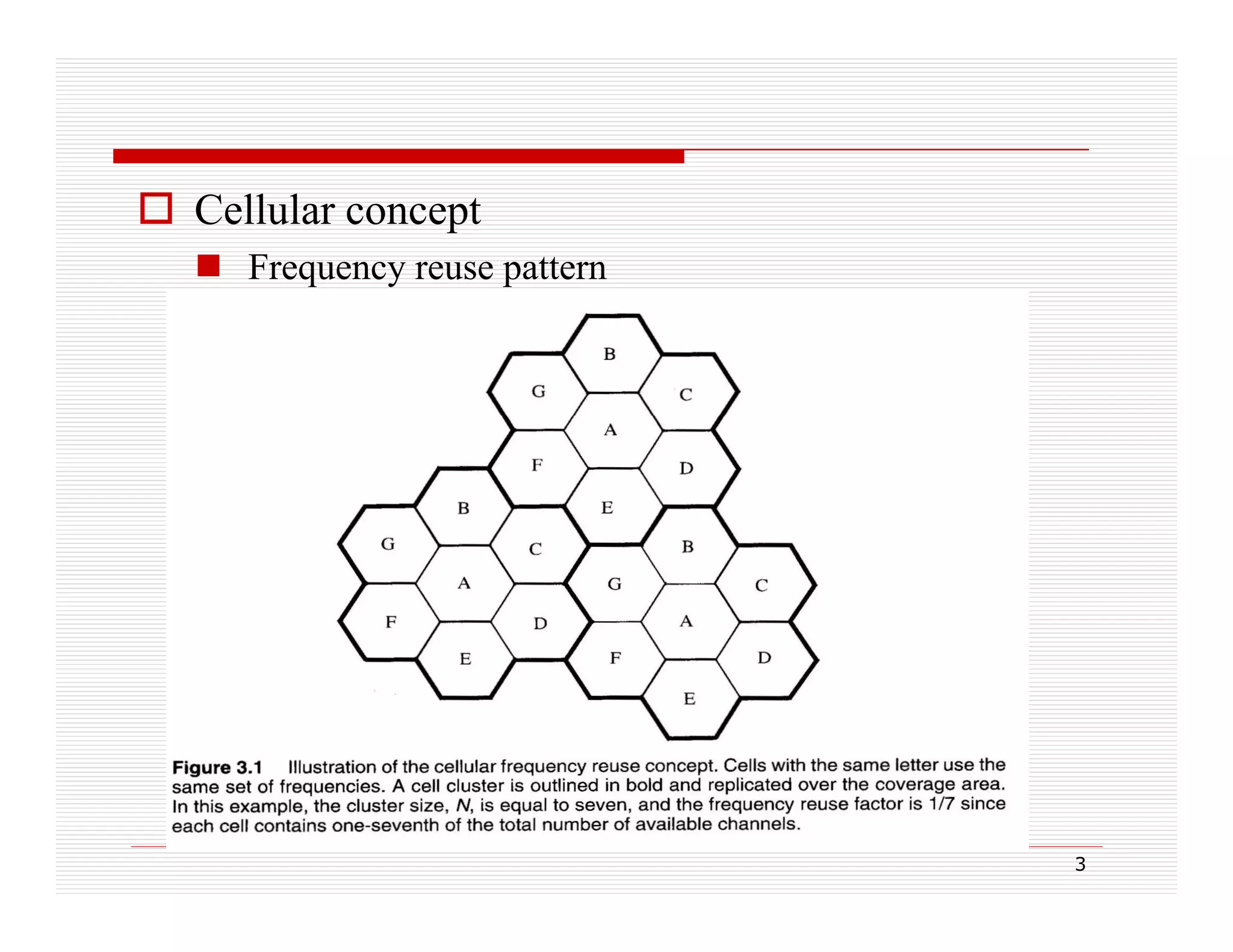
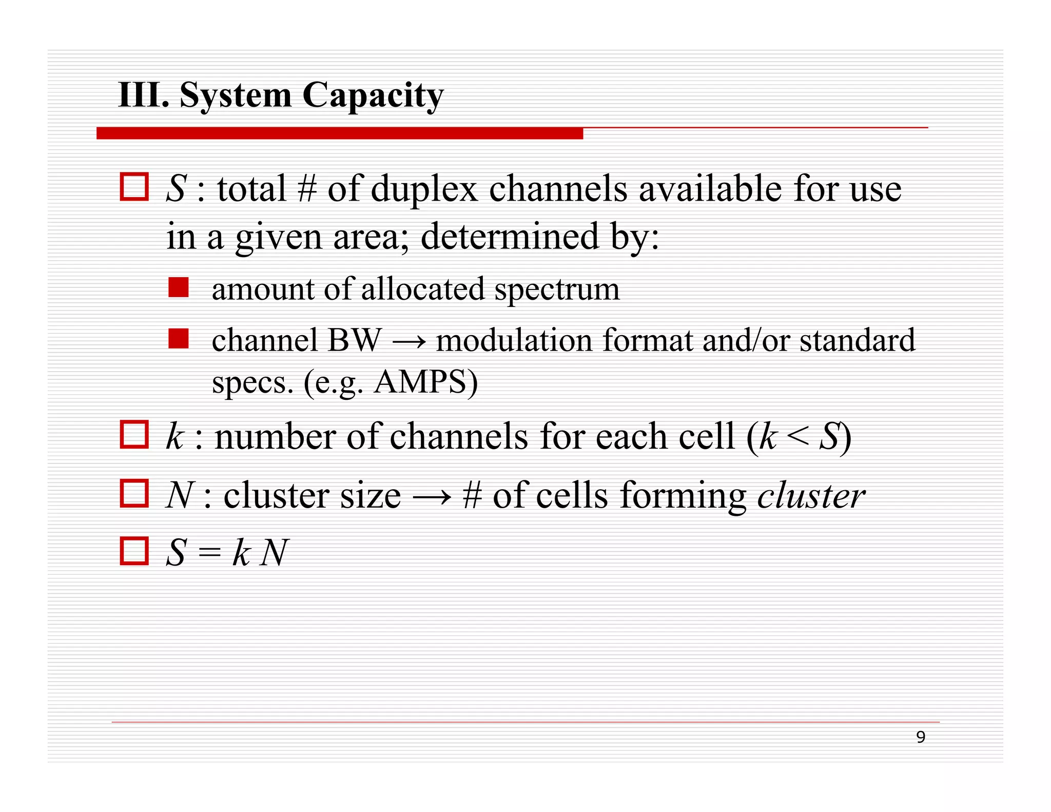
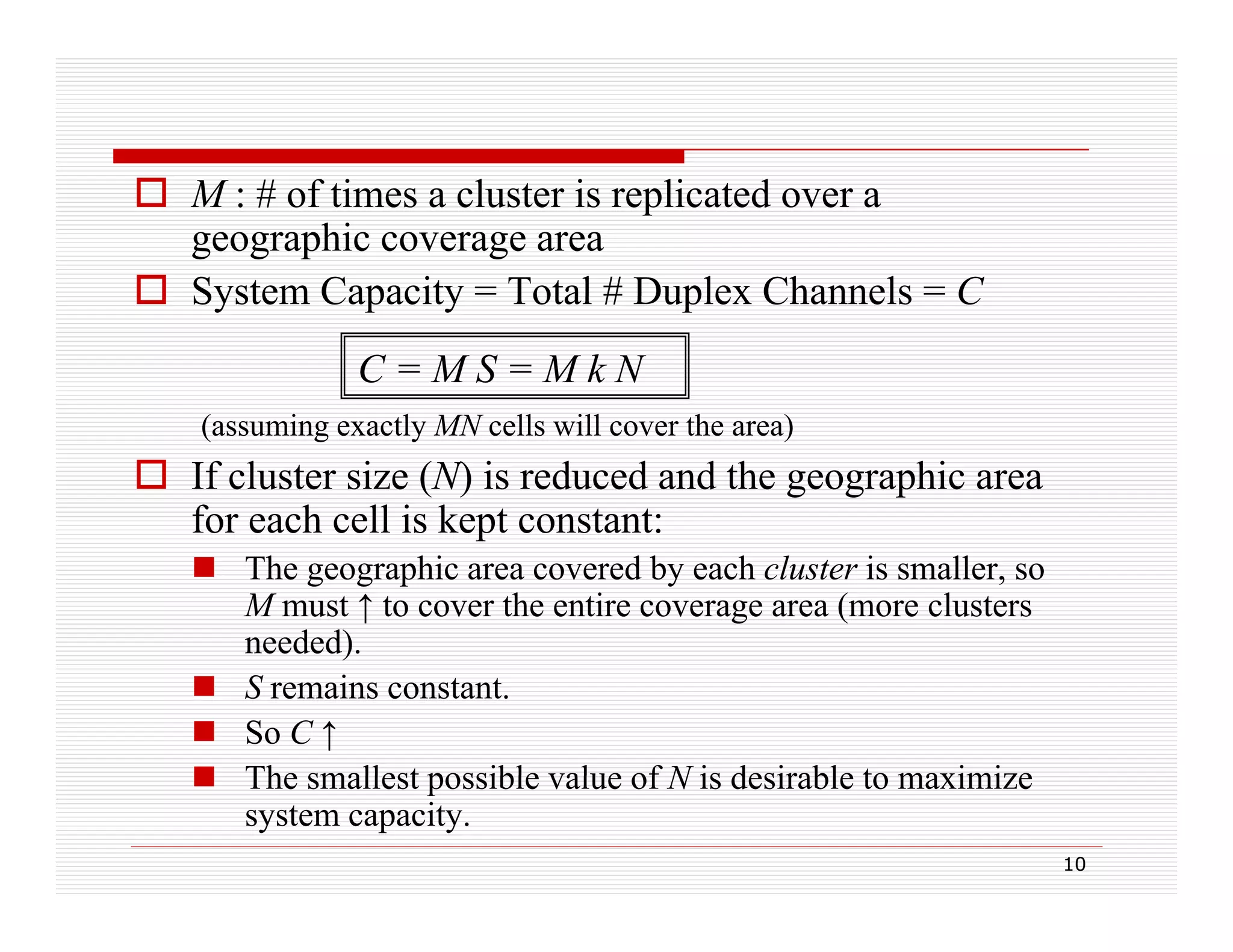
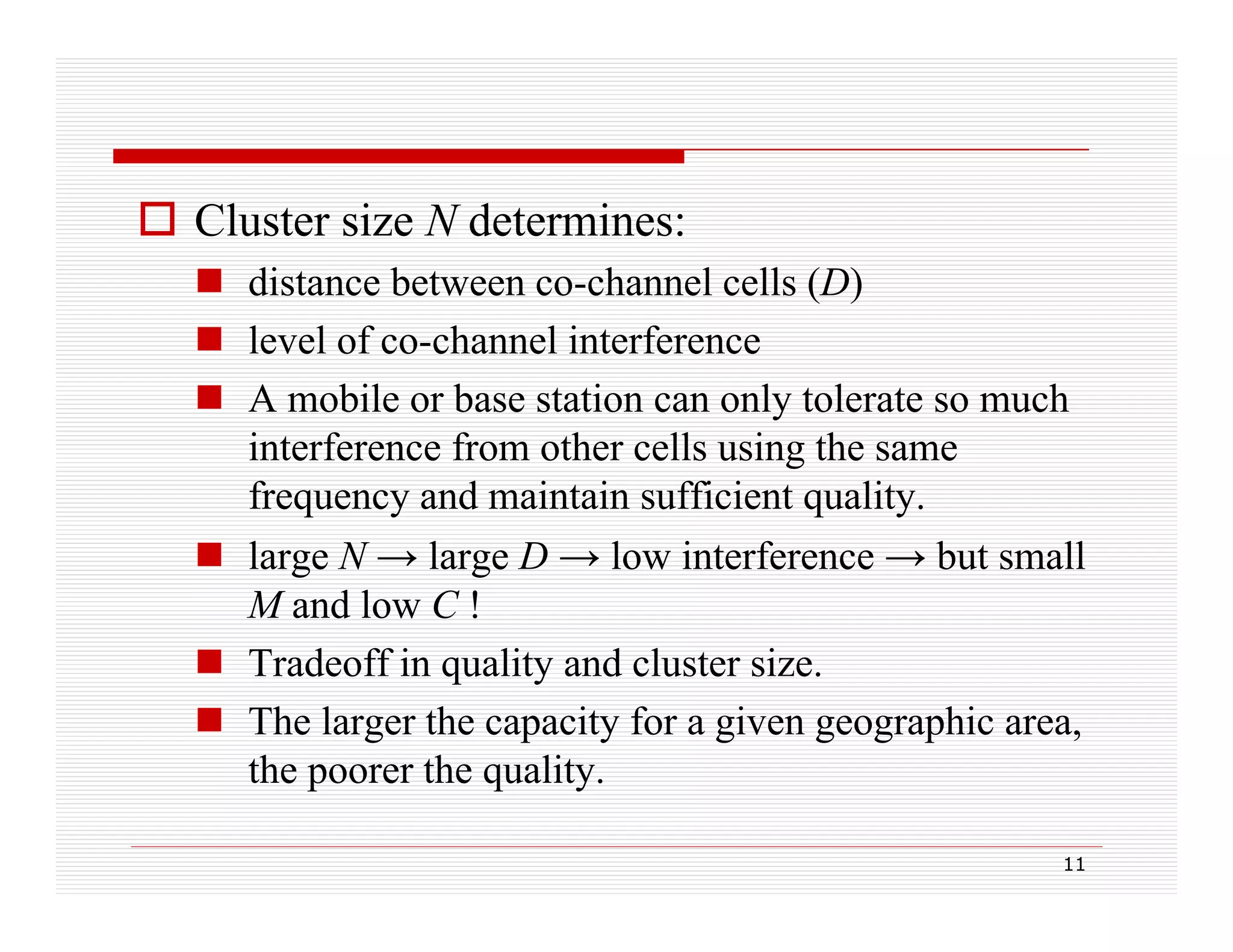
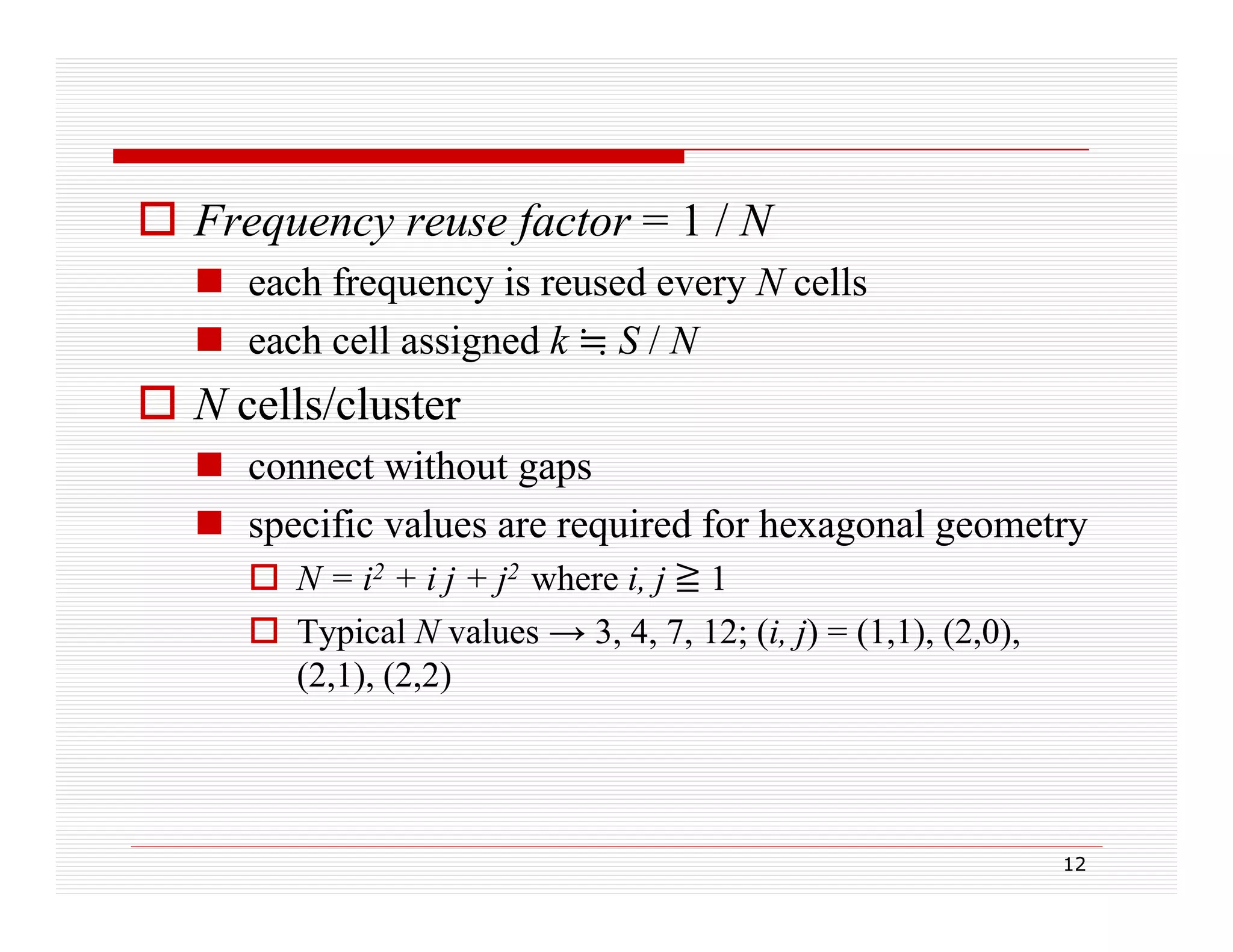
The document discusses key concepts in cellular system design including frequency reuse, cell size, system capacity, and handoff strategies. The cellular concept allows efficient reuse of a fixed number of channels across a large coverage area by dividing the area into smaller cells and reusing frequencies in cells sufficiently distant from each other to prevent interference. System capacity is determined by the number of available channels, cluster size which impacts frequency reuse distance and interference levels, and the number of times a cluster can be replicated across the coverage area. Handoff strategies aim to transfer calls seamlessly between cells as users move and involve monitoring signal levels, assigning priority to handoffs over new calls, and reserving guard channels.


![Vibe Coding vs. Spec-Driven Development [Free Meetup]](https://cdn.slidesharecdn.com/ss_thumbnails/vibecodingvsspecdrivendevelopment-251209105622-43f455e7-thumbnail.jpg?width=640&height=640&fit=bounds)


