Download as PDF, PPTX


![Warm up example
Data set
import pandas as pd
data = {’age’: [38, 49, 27, 19, 54, 29, 19, 42, 34, 64,
19, 62, 27, 77, 55, 41, 56, 32, 59, 35],
’distance’: [6169.98, 7598.87, 3276.07, 1570.43, 951.76,
139.97, 4476.89, 8958.77, 1336.44, 6138.85,
2298.68, 1167.92, 676.30, 736.85, 1326.52,
712.13, 3083.07, 1382.64, 2267.55, 2844.18],
’attended’: [False, False, False, True, True, True, False,
True, True, True, False, True, True, True,
False, True, True, True, True, False]}
df = pd.DataFrame(data)
age distance attended
0 38 6169.98 False
1 49 7598.87 False
2 27 3276.07 False
3 19 1570.43 True
4 54 951.76 True
5 29 139.97 True
6 19 4476.89 False
7 42 8958.77 True
8 34 1336.44 True
9 64 6138.85 True
10 19 2298.68 False
11 62 1167.92 True
7 / 47
CART: Not only Classification and Regression Trees - Marc Garcia](https://image.slidesharecdn.com/cart-160312161201/75/CART-Not-only-Classification-and-Regression-Trees-7-2048.jpg)
![Warm up example
Data set visualization
from bokeh.plotting import figure, show
p = figure(title = ’Event attendance’)
p.xaxis.axis_label = ’Distance’
p.yaxis.axis_label = ’Age’
p.circle(df[df.attended][’distance’],
df[df.attended][’age’],
color=’red’,
legend=’Attended’,
fill_alpha=0.2,
size=10)
p.circle(df[~df.attended][’distance’],
df[~df.attended][’age’],
color=’blue’,
legend="Didn’t attend",
fill_alpha=0.2,
size=10)
show(p)
8 / 47
CART: Not only Classification and Regression Trees - Marc Garcia](https://image.slidesharecdn.com/cart-160312161201/75/CART-Not-only-Classification-and-Regression-Trees-8-2048.jpg)
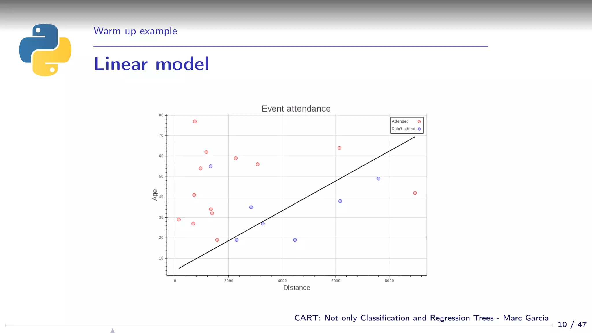
![Warm up example
Using a linear model
from sklearn.linear_model import LogisticRegression
logit = LogisticRegression()
logit.fit(df[[’age’, ’distance’]], df[’attended’])
def get_y(x): return -(logit.intercept_[0] + logit.coef_[0,1] * x) / logit.coef_[0,0]
plot = base_plot()
min_x, max_x = df[’distance’].min(), df[’distance’].max()
plot.line(x=[min_x, max_x],
y=[get_y(min_x), get_y(max_x)],
line_color=’black’,
line_width=2)
_ = show(plot)
9 / 47
CART: Not only Classification and Regression Trees - Marc Garcia](https://image.slidesharecdn.com/cart-160312161201/75/CART-Not-only-Classification-and-Regression-Trees-9-2048.jpg)

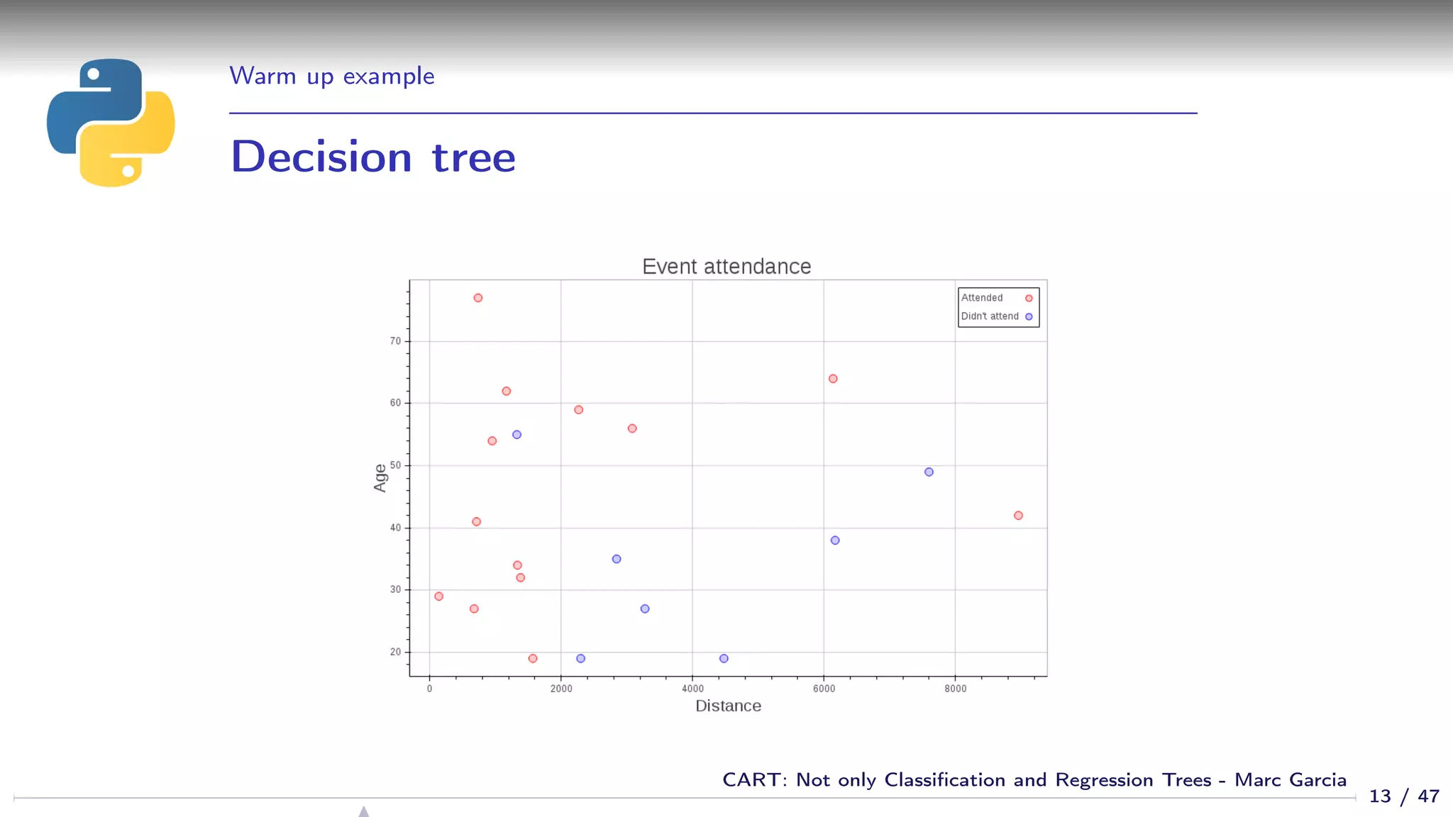
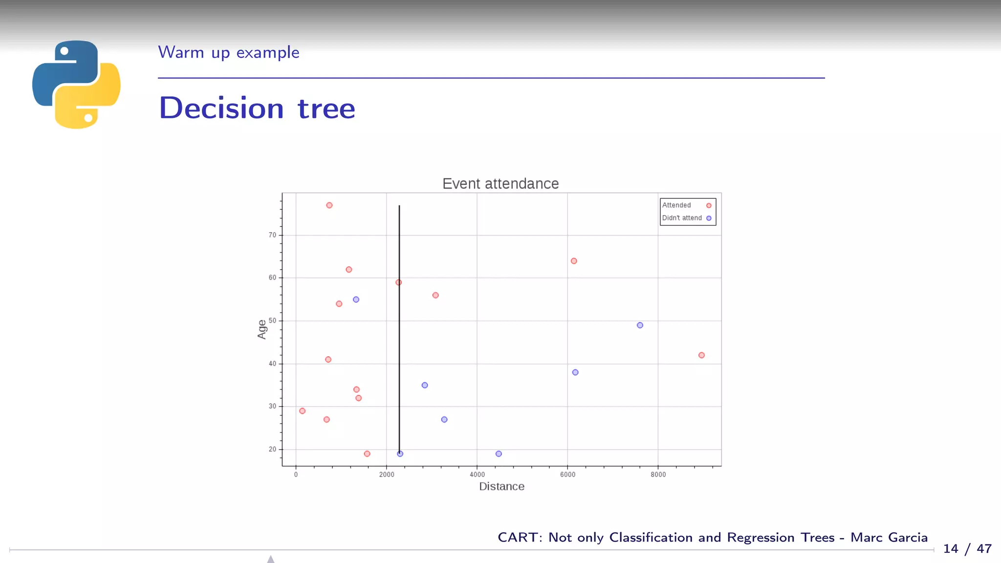
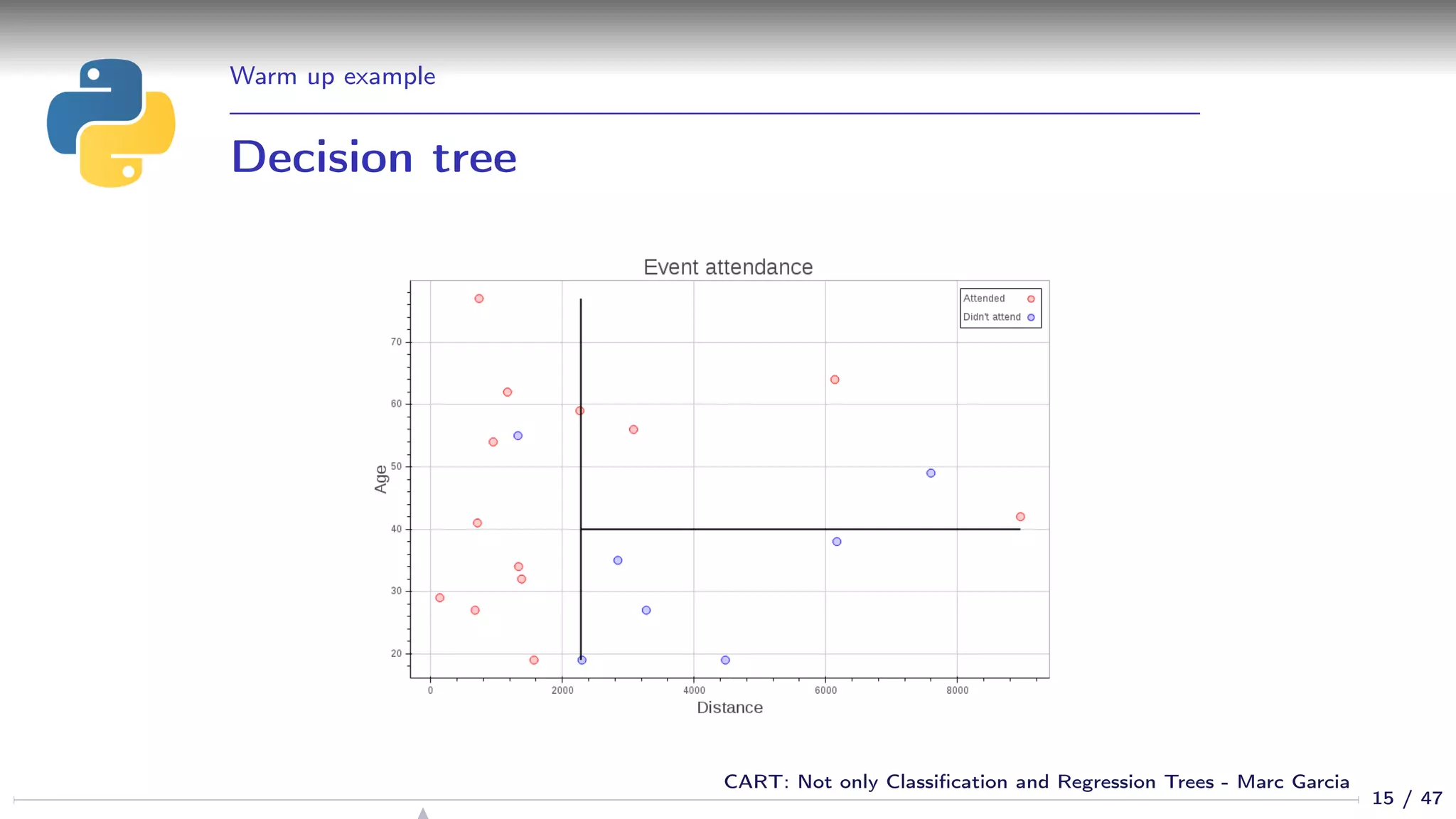
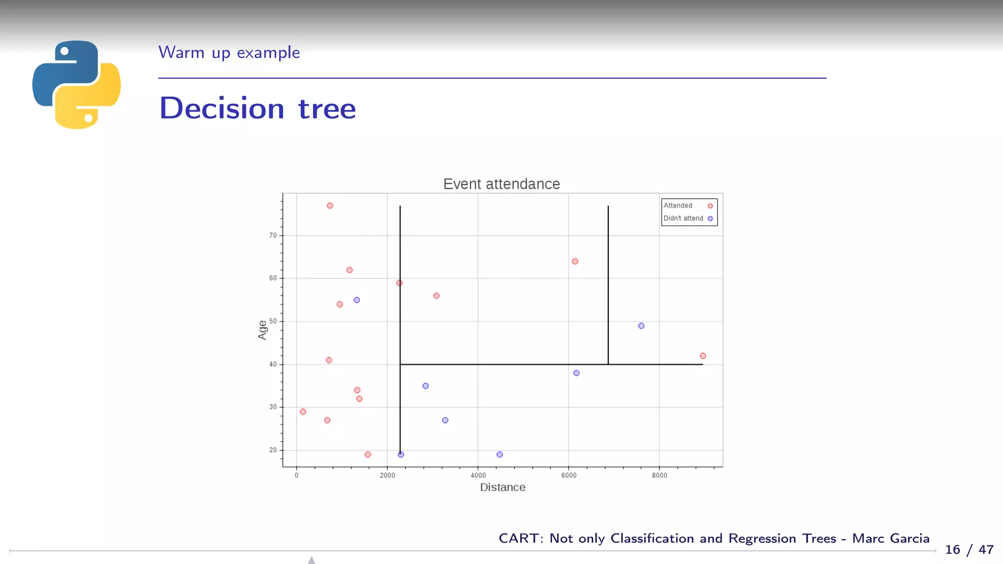
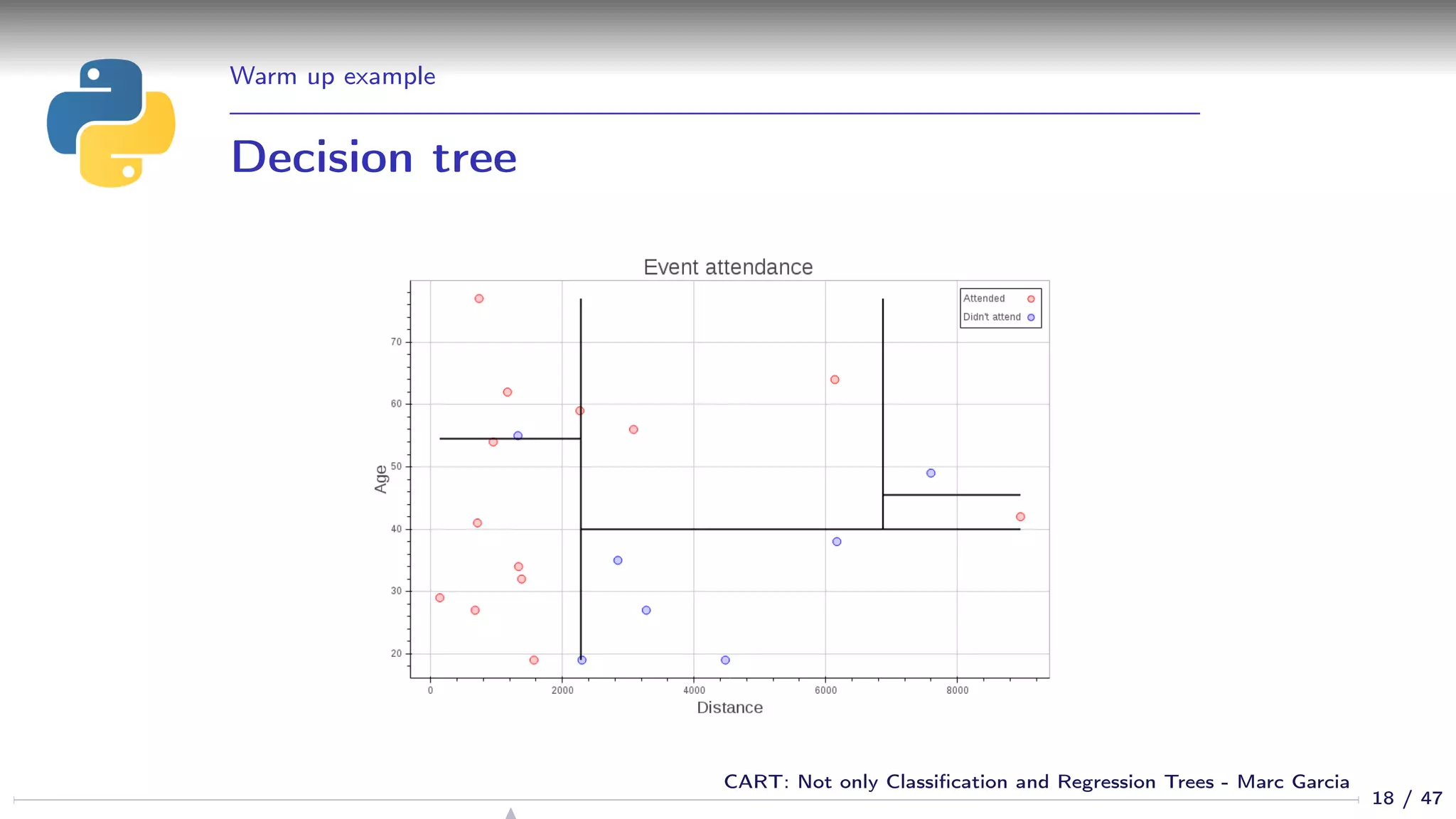
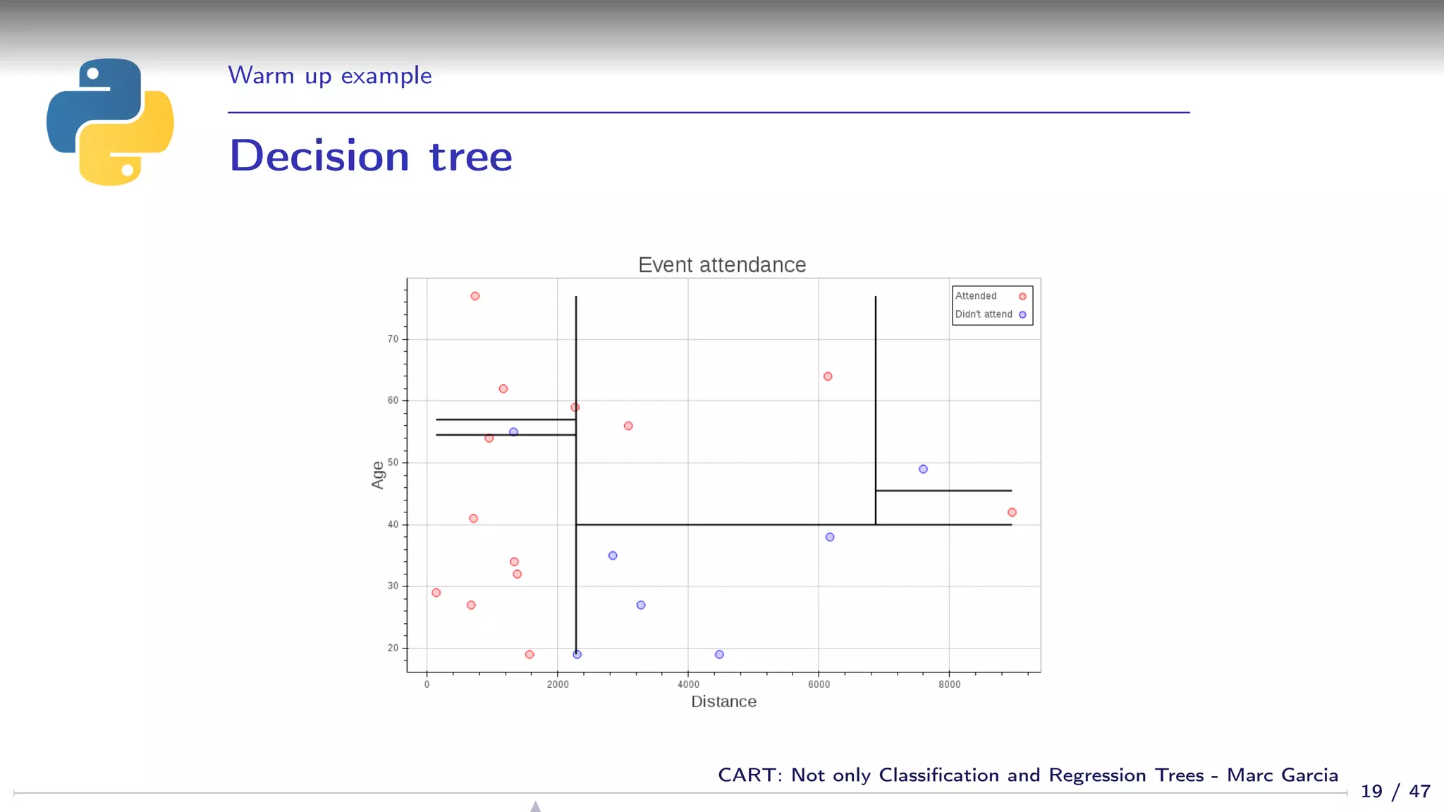
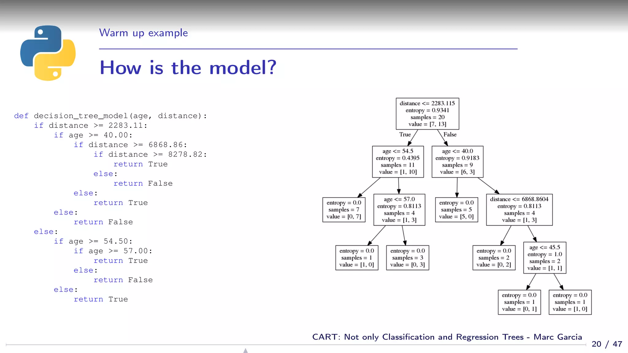
![Warm up example
Using a decision tree
from sklearn.tree import DecisionTreeClassifier
dtree = DecisionTreeClassifier()
dtree.fit(df[[’age’, ’distance’]], df[’attended’])
cart_plot(dtree)
12 / 47
CART: Not only Classification and Regression Trees - Marc Garcia](https://image.slidesharecdn.com/cart-160312161201/75/CART-Not-only-Classification-and-Regression-Trees-12-2048.jpg)


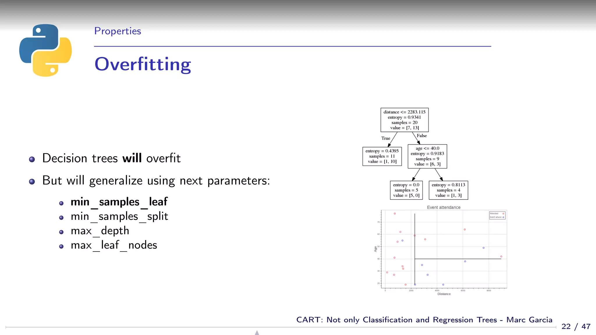

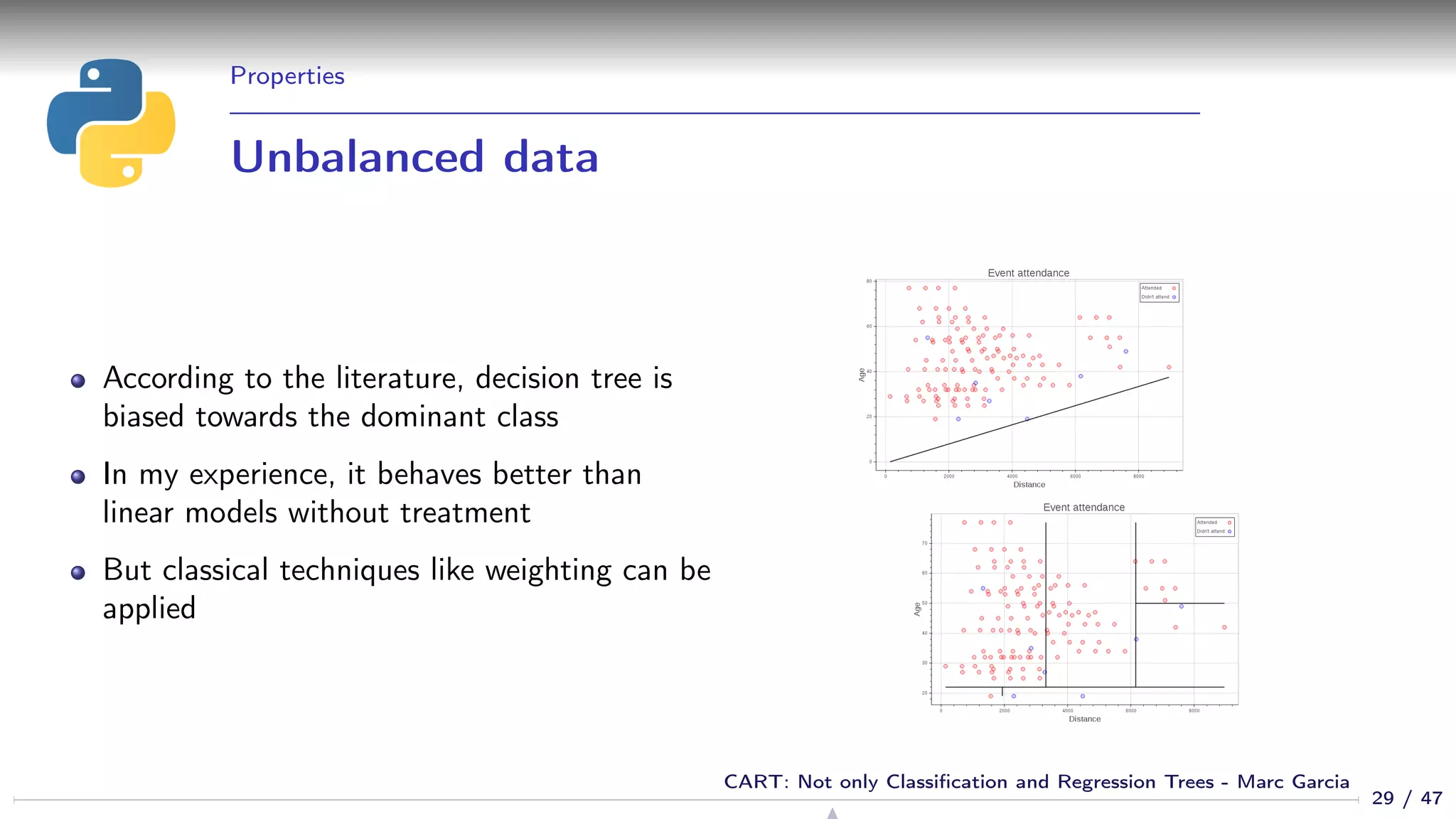
![Properties
Feature selection
We get feature selection for free
If a feature is not relevant, it is not used in the tree
sklearn: Gives you the feature importances:
>>> list(zip([’age’, ’distance’],
... dtree.feature_importances_))
[(’age’, 0.5844155844155845), (’distance’, 0.41558441558441556)]
25 / 47
CART: Not only Classification and Regression Trees - Marc Garcia](https://image.slidesharecdn.com/cart-160312161201/75/CART-Not-only-Classification-and-Regression-Trees-25-2048.jpg)


![Training
Basic algorithm
def train_decision_tree(x, y):
feature, value = get_best_split(x, y)
x_left, y_left = x[x[feature] < value], y[x[feature] < value]
if len(y_left.unique()) > 1:
left_node = train_decision_tree(x_left, y_left)
else:
left_node = None
x_right, y_right = x[x[feature] >= value], y[x[feature] >= value]
if len(y_right.unique()) > 1:
right_node = train_decision_tree(x_right, y_right)
else:
right_node = None
return Node(feature, value, left_node, right_node)
33 / 47
CART: Not only Classification and Regression Trees - Marc Garcia](https://image.slidesharecdn.com/cart-160312161201/75/CART-Not-only-Classification-and-Regression-Trees-33-2048.jpg)
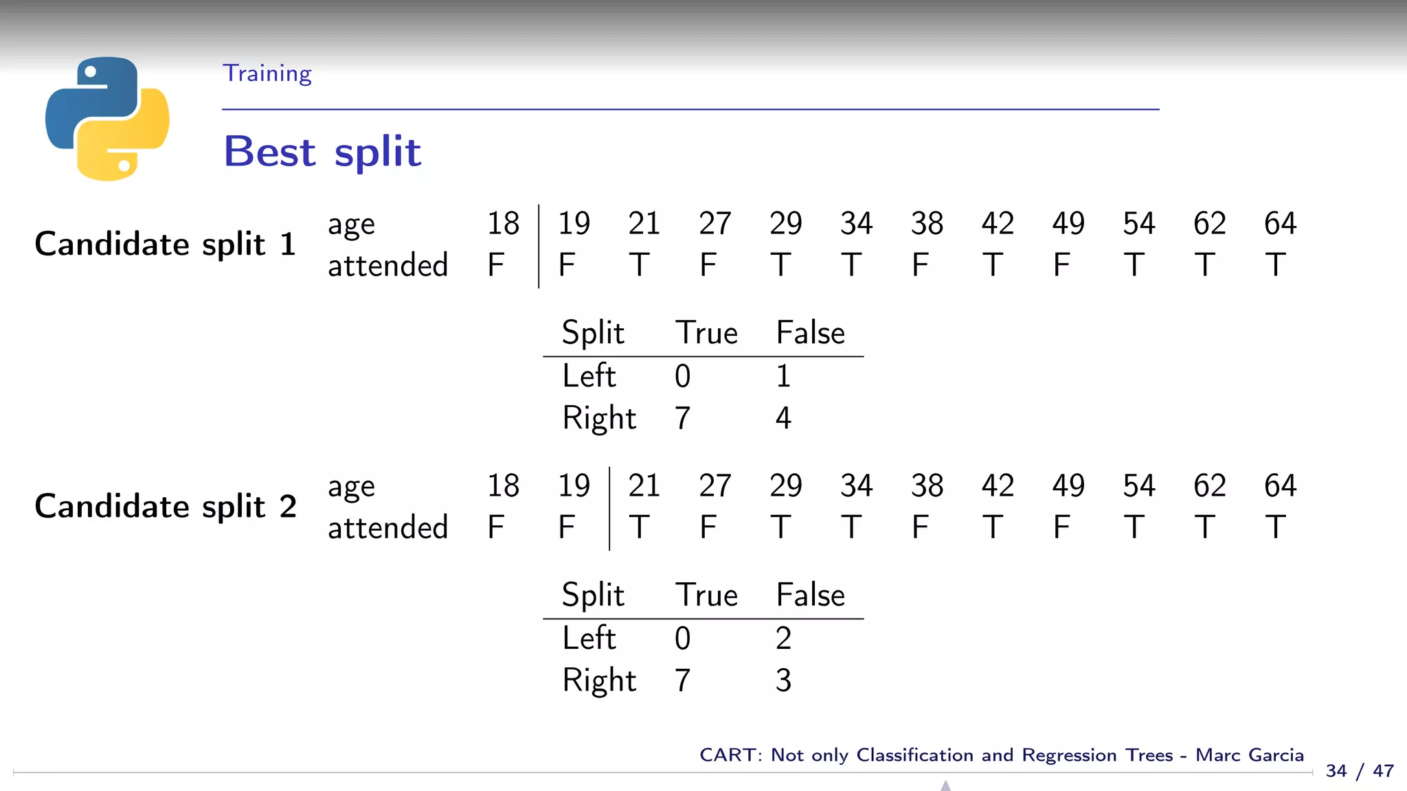
![Training
Best split algorithm
def get_best_split(x, y):
best_split = None
best_entropy = 1.
for feature in x.columns.values:
column = x[feature]
for value in column.iterrows():
a = y[column < value] == class_a_value
b = y[column < value] == class_b_value
left_weight = (a + b) / len(y.index)
left_entropy = entropy(a, b)
a = y[column >= value] == class_a_value
b = y[column >= value] == class_b_value
right_items = (a + b) / len(y.index)
right_entropy = entropy(a, b)
split_entropy = left_weight * left_etropy + right_weight * right_entropy
if split_entropy < best_entropy:
best_split = (feature, value)
best_entropy = split_entropy
return best_split
35 / 47
CART: Not only Classification and Regression Trees - Marc Garcia](https://image.slidesharecdn.com/cart-160312161201/75/CART-Not-only-Classification-and-Regression-Trees-35-2048.jpg)


![Appendix
CART plot decision boundaries (I)
from collections import namedtuple, deque
from functools import partial
class NodeRanges(namedtuple(’NodeRanges’, ’node,max_x,min_x,max_y,min_y’)):
pass
def cart_plot(nodes):
nodes = tree_to_nodes(dtree)
plot = base_plot()
add_line = partial(plot.line, line_color=’black’, line_width=2)
stack = deque()
stack.append(NodeRanges(node=nodes[0],
max_x=df[’distance’].max(),
min_x=df[’distance’].min(),
max_y=df[’age’].max(),
min_y=df[’age’].min()))
# (continues)
45 / 47
CART: Not only Classification and Regression Trees - Marc Garcia](https://image.slidesharecdn.com/cart-160312161201/75/CART-Not-only-Classification-and-Regression-Trees-45-2048.jpg)
![Appendix
CART plot decision boundaries (II)
while len(stack):
node, max_x, min_x, max_y, min_y = stack.pop()
feature, threshold, left, right = node
if feature == ’distance’:
add_line(x=[threshold, threshold], y=[min_y, max_y])
elif feature == ’age’:
add_line(x=[min_x, max_x], y=[threshold, threshold])
else:
continue
stack.append(NodeRanges(node=nodes[left],
max_x=threshold if feature == ’distance’ else max_x,
min_x=min_x,
max_y=threshold if feature == ’age’ else max_y,
min_y=min_y))
stack.append(NodeRanges(node=nodes[right],
max_x=max_x,
min_x=threshold if feature == ’distance’ else min_x,
max_y=max_y,
min_y=threshold if feature == ’age’ else min_y))
show(plot)
46 / 47
CART: Not only Classification and Regression Trees - Marc Garcia](https://image.slidesharecdn.com/cart-160312161201/75/CART-Not-only-Classification-and-Regression-Trees-46-2048.jpg)


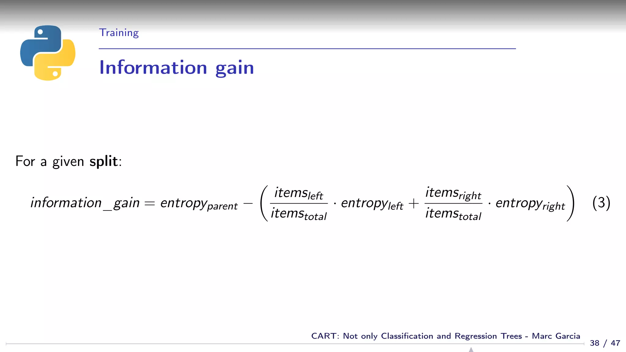
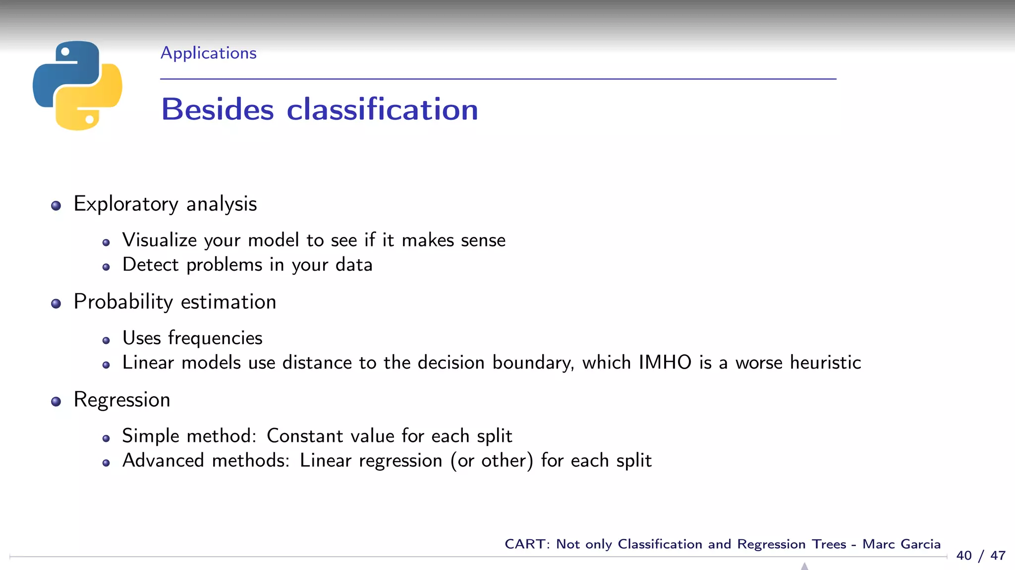
The document provides an overview of Classification and Regression Trees (CART) presented by Marc Garcia, focusing on how decision trees operate, their advantages, common issues, and applications for classification. It discusses training techniques, model evaluation, and properties such as overfitting, handling of categorical variables, and performance compared to linear models. Examples are provided to illustrate data visualization, modeling with logistic regression and decision trees, along with methods for feature selection and model debugging.


![Vibe Coding vs. Spec-Driven Development [Free Meetup]](https://cdn.slidesharecdn.com/ss_thumbnails/vibecodingvsspecdrivendevelopment-251209105622-43f455e7-thumbnail.jpg?width=640&height=640&fit=bounds)


