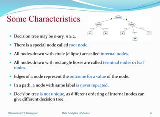
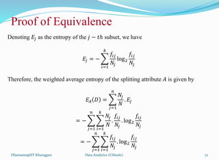
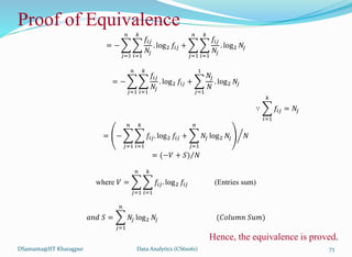
This document discusses decision tree induction and the concept of entropy. It begins with an overview of decision trees, how they are used for classification tasks, and the basic algorithm for building a decision tree from a training dataset. It then covers node splitting for different attribute types in more detail. Examples are provided to illustrate decision tree building. The document also discusses the concept of entropy from information theory and how it is used as a measure of uncertainty in a training dataset to select the best attributes during decision tree construction.


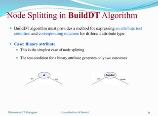
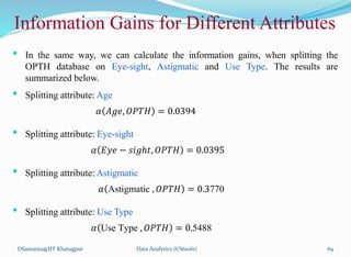
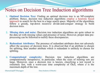
![Illustration : BuildDT Algorithm
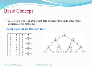
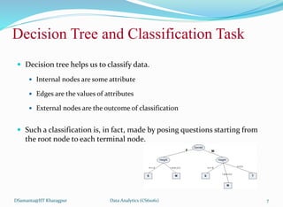
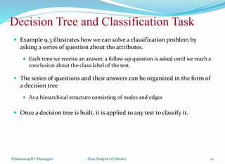
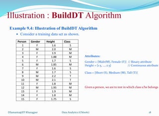
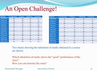
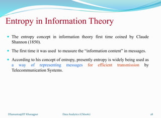
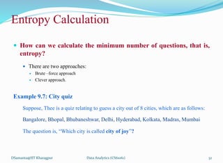
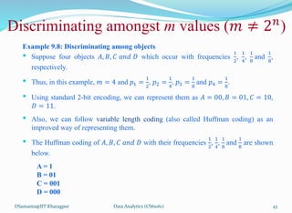
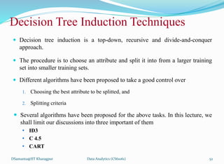
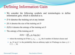
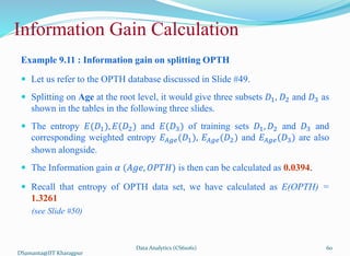
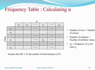
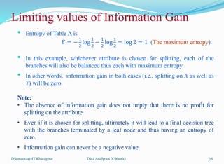
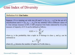
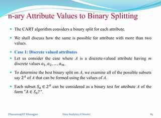
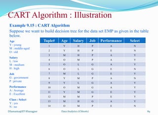
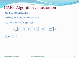
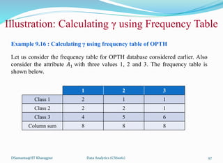
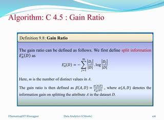
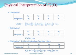
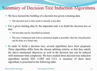
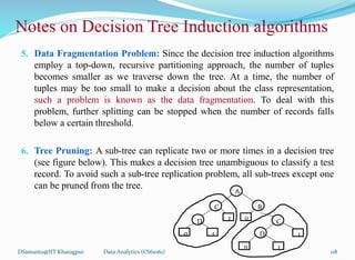
Example 9.5: Illustration of BuildDT Algorithm
Consider an anonymous database as shown.
DSamanta@IIT Kharagpur
A1 A2 A3 A4 Class
a11 a21 a31 a41 C1
a12 a21 a31 a42 C1
a11 a21 a31 a41 C1
a11 a22 a32 a41 C2
a11 a22 a32 a41 C2
a12 a22 a31 a41 C1
a11 a22 a32 a41 C2
a11 a22 a31 a42 C1
a11 a21 a32 a42 C2
a11 a22 a32 a41 C2
a12 a22 a31 a41 C1
a12 a22 a31 a42 C1
• Is there any “clue” that enables to
select the “best” attribute first?
• Suppose, following are two
attempts:
• A1A2A3A4 [Naïve]
• A3A2A4A1 [Random]
• Draw the decision trees in the above-
mentioned two cases.
• Are the trees different to classify any test
data?
• If any other sample data is added into the
database, is that likely to alter the decision
tree already obtained?
Data Analytics (CS61061) 22](https://image.slidesharecdn.com/09decisiontreeinduction-240217052000-2a8009b3/85/About-decision-tree-induction-which-helps-in-learning-22-320.jpg)
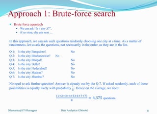
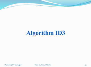
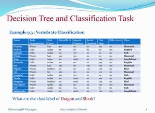
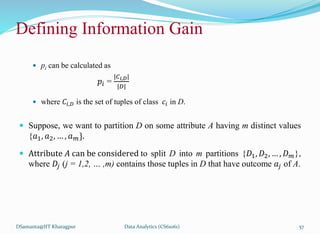
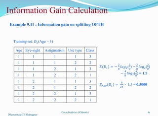
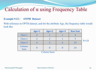
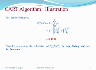
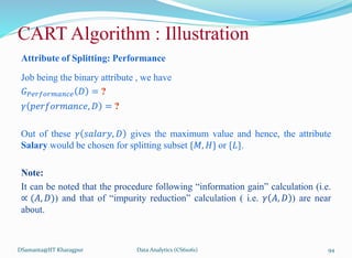
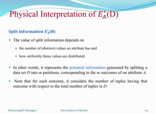
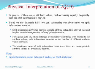
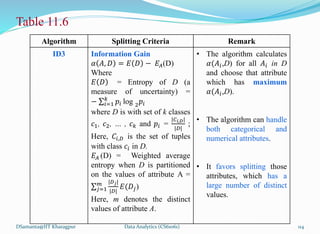
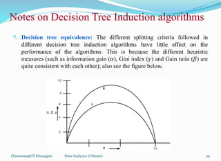
![ID3: Decision Tree Induction Algorithms
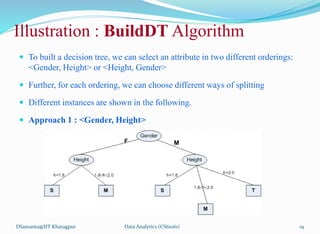
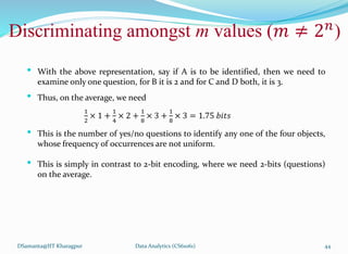
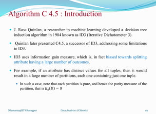
Quinlan [1986] introduced the ID3, a popular short form of Iterative
Dichotomizer 3 for decision trees from a set of training data.
In ID3, each node corresponds to a splitting attribute and each arc is a
possible value of that attribute.
At each node, the splitting attribute is selected to be the most informative
among the attributes not yet considered in the path starting from the root.
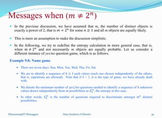
DSamanta@IIT Kharagpur Data Analytics (CS61061) 54](https://image.slidesharecdn.com/09decisiontreeinduction-240217052000-2a8009b3/85/About-decision-tree-induction-which-helps-in-learning-54-320.jpg)


![제 23회 보아즈(BOAZ) 빅데이터 컨퍼런스 - [MBOAX] : ABSA를 활용한 소비자 반응 분석 기반 운영 효율화 대시보드 설계](https://cdn.slidesharecdn.com/ss_thumbnails/3-1boaz23rdconferencemboax-260203102709-9d519923-thumbnail.jpg?width=640&height=640&fit=bounds)


