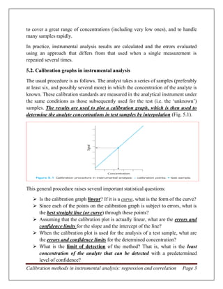
Calibration methods in instrumental analysis: regression and correlation Page 1
Calibration methods in instrumental analysis: regression and correlation
5.1. Introduction: instrumental analysis
Classical or ‘wet chemistry’ analysis techniques such as titrimetry and gravimetry
remain in use in many laboratories. They are ideal for high-precision analyses,
especially when small numbers of samples are involved, and are sometimes
necessary for the analysis of standard materials. In practice, however, almost all
analyses are now performed using instrumental methods. Techniques using
absorption and emission spectrometry at various wavelengths, electrochemistry,
mass spectrometry, chromatographic and electrophoretic separations, thermal and
radiochemical methods probably account for at least 90% of all current analytical
work. There are several reasons for this. Instrumental methods can perform
analyses that are difficult or impossible by classical methods. The latter can only
rarely detect materials at sub-microgram levels, while instrumental methods can
provide the ultimate in terms of sensitivity: in recent years fluorescence and
electrochemical methods have been used to detect single organic molecules in very
small volumes of solution. While ‘wet chemical’ methods can usually determine
only one analyte at a time, many instrumental methods have multi-analyte
capability, especially with the aid of modern chemometrics to interpret the data.
Most classical methods only operate over a concentration range of two to three
orders of magnitude (i.e. powers of 10), but many instrumental techniques work
well over a range of six or more orders of magnitude: this characteristic has
important implications for the statistical treatment of the results.
When there are many samples to be analysed instrumental methods are generally
quicker and often cheaper than the labour-intensive manual methods. In clinical
analysis, for example, there is frequently a requirement for the same analyses to be
done on scores or even hundreds of whole blood or blood serum/plasma samples
every day. Despite the high initial cost of the equipment, such work is generally
performed using completely automatic systems. Automation has become such an
important feature of analytical chemistry that the ease with which a particular
technique can be automated often determines whether or not it is used. A typical
automatic method may be able to process samples at the rate of 100 per hour or
more.
Calibration methods in instrumental analysis: regression and correlation Page 2
The equipment will take a measured volume of sample, dilute it appropriately,
conduct one or more reactions with it, and determine and record the concentration
of the analyte or of a derivative produced in the reactions.
Other areas where the use of automated equipment is now crucial include
environmental monitoring and the rapidly growing field of industrial process
analysis. Special problems of error estimation will evidently arise in all these
applications of automatic analysis: systematic errors, for example, must be
identified and corrected as rapidly as possible. An important trend in modern
instrumental analysis is the development of miniaturised systems, which often
combine modern micro-electronic components with micro-fluidic sample handling
systems. Such tiny analytical systems have great potential in process analysis, in
vivo diagnostics, security-related detection systems and many other areas.
Lastly, modern analytical instruments are invariably interfaced with personal
computers to provide sophisticated system control, and the storage, treatment and
reporting of data. Such systems can also evaluate the results statistically, and
compare the analytical results with data libraries so as to match spectral and other
information. All these facilities are now available from low-cost computers
operating at high speeds. Also important is the use of ‘intelligent’ instruments,
which incorporate automatic set-up and fault diagnosis and can perform
optimization processes.
Instrumental analysis methods – why?
 Extreme sensitivity, ability to measure very small changes, sometimes single
molecule detection.
 Very wide concentration ranges.
 Multi-analyte capability in conjunction with suitable data handling.
 Automation: high sample throughput and low cost per sample.
 Miniaturised systems.
 Computer interfacing for control, rapid data handling, optimisation.
The statistical procedures used with instrumental analysis methods must provide,
as always, information on the precision and accuracy of the measurements. They
must also reflect the technical advantages of such methods, especially their ability
Calibration methods in instrumental analysis: regression and correlation Page 3
to cover a great range of concentrations (including very low ones), and to handle
many samples rapidly.
In practice, instrumental analysis results are calculated and the errors evaluated
using an approach that differs from that used when a single measurement is
repeated several times.
5.2. Calibration graphs in instrumental analysis
The usual procedure is as follows. The analyst takes a series of samples (preferably
at least six, and possibly several more) in which the concentration of the analyte is
known. These calibration standards are measured in the analytical instrument under
the same conditions as those subsequently used for the test (i.e. the ‘unknown’)
samples. The results are used to plot a calibration graph, which is then used to
determine the analyte concentrations in test samples by interpolation (Fig. 5.1).
This general procedure raises several important statistical questions:
 Is the calibration graph linear? If it is a curve, what is the form of the curve?
 Since each of the points on the calibration graph is subject to errors, what is
the best straight line (or curve) through these points?
 Assuming that the calibration plot is actually linear, what are the errors and
confidence limits for the slope and the intercept of the line?
 When the calibration plot is used for the analysis of a test sample, what are
the errors and confidence limits for the determined concentration?
 What is the limit of detection of the method? That is, what is the least
concentration of the analyte that can be detected with a predetermined
level of confidence?
Calibration methods in instrumental analysis: regression and correlation Page 4
Before tackling these questions in detail, we must consider a number of aspects
of plotting calibration graphs. First, it is usually essential that the calibration
standards cover the whole range of concentrations required in the subsequent
analyses. With the important exception of the ‘method of standard additions’,
which is treated separately in a later section, concentrations of test samples are
normally determined by interpolation and not by extrapolation. Second, it is
crucially important to include the value for a ‘blank’ sample in the calibration
curve. The blank contain no deliberately added analyte, but does contain the
same solvent, reagents, etc., as the other test samples, and is subjected to
exactly the same sequence of analytical procedures. The instrument signal
given by the blank sample will sometimes not be zero. This signal is subject to
errors like all the other points on the calibration plot, so it is wrong in principle
to subtract the blank value from the other standard values before plotting the
calibration graph. This is because when two quantities are subtracted, the
error in the final result cannot also be obtained by simple subtraction.
Subtracting the blank value from each of the other instrument signals before
plotting the graph thus gives incorrect information on the errors in the
calibration process.
Several assumptions are implicit in the usual methods for plotting calibration
graphs. The calibration curve is always plotted with the instrument signals on
the vertical (y) axis and the standard concentrations on the horizontal (x)
axis. This is because many of the procedures to be described in the following
sections assume that all the errors are in the y-values and that the standard
concentrations (x-values) are error-free. In many routine instrumental analyses
this assumption may well be justified. The standards can usually be made up
with an error of ca. 0.1% or better, whereas the instrumental measurements
themselves might have a coefficient of variation of 1–3% or worse. So the x-
axis error is indeed negligible compared with the y-axis one. In recent years,
however, the advent of high-precision automatic methods with coefficients of
variation of 0.5% or better has put the assumption under question, and has led
some users to make up their standard solutions by weight rather than by the
less accurate combination of weight and volume. This approach is intended to
ensure that the x-axis errors remain small compared with the y-axis ones. If for
any reason this assumption is not valid, then separate, though more complex,
approaches to plotting the calibration graph are available.
Calibration methods in instrumental analysis: regression and correlation Page 5
Other common assumptions are that if several measurements are made on a
given standard material, the y-values obtained have a normal (Gaussian) error
distribution, and that the magnitude of the random errors in the y-values is
independent of the analyte concentration. The first of these two assumptions is
normally sound, but the second requires further discussion. If true, it implies
that all the points on the graph should have equal weight in our calculations, i.e.
that it is equally important for the line to pass close to points with high y-values
and to those with low y-values. Such calibration graphs are said to be weighted,
and are treated. However, in practice the y-value errors often increase as the
analyte concentration increases. This means that the calibration points should
have unequal weights in our calculation, as it is more important for the line to
pass close to the points where the errors are least. These weighted calculations
are now becoming more common despite their additional complexity. In
subsequent sections we shall assume that straight line calibration graphs take
the algebraic form:
Where b is the slope of the line and a is its intercept on the y-axis. The
individual points on the line will be referred to as (x1, y1 – normally the ‘blank’
reading), (x2, y2), (x3, y3) . . . (xi, yi) . . . (xn, yn), i.e. there are n points
altogether. The mean of the x-values is, as usual, called and the mean of the
y-values is the position is then known as the ‘centroid’ of all the
points.
5.3. The product–moment correlation coefficient
Is the calibration plot linear? A common method of estimating how well the
experimental points fit a straight line is to calculate the product–moment
correlation coefficient, r. This statistic is often referred to simply as the
‘correlation coefficient’ because in quantitative sciences it is much more
commonly used than the other types of correlation coefficient.
Calibration methods in instrumental analysis: regression and correlation Page 6
The value of r is given by:
It can be shown that r can only take values in the range . As
indicated in Fig. 5.2, an r value of -1 describes perfect negative correlation, i.e.
all the experimental points lie on a straight line of negative slope. Similarly,
when r=+1 we have perfect positive correlation, all the points lying exactly on a
straight line of positive slope. When there is no linear correlation between x and
y the value of r is close to zero. In analytical practice, calibration graphs
frequently give numerical r-values greater than 0.99, and r values less than
about 0.90 are relatively uncommon. A typical example of a calculation of r
illustrates a number of important points.
Calibration methods in instrumental analysis: regression and correlation Page 7
As we have seen, r-values obtained in instrumental analysis are normally very
high, so a calculated value, together with the calibration plot itself, is often
sufficient to assure the analyst that a useful linear relationship has been
obtained. In some circumstances, however, much lower r-values are obtained:
one such situation is further discussed in Section 5.9. In these cases it will be
necessary to use a proper statistical test to see whether the correlation
coefficient is significant, bearing in mind the number of points used in the
calculation. The simplest method of doing this is to calculate a t-value using the
following equation:
The calculated value of t is compared with the tabulated value at the desired
significance level, using a two-sided t-test and (n – 2) degrees of freedom. The
null hypothesis in this case is that there is no correlation between x and y. If the
calculated value of t is greater than the tabulated value, the null hypothesis is
rejected and we conclude that a significant correlation does exist. As expected,
the closer |r| is to 1, i.e. as the straight line relationship becomes stronger, the
larger the values of t that are obtained.
5.4. The line of regression of y on x
In this section we assume that there is a linear relationship between the
analytical signal (y) and the concentration (x), and show how to calculate the
‘best’ straight line through the calibration graph points, each of which is
subject to experimental error. Since we are assuming for the present that all the
errors are in y, we are seeking the line that minimizes the deviations in the y-
direction between the experimental points and the calculated line. Since some
of these deviations (technically known as the y-residuals) will be positive and
some negative, it is sensible to try to minimize the sum of the squares of the
residuals, since these squares will all be positive. This explains the frequent use
of the term method of least squares for the procedure.
Calibration methods in instrumental analysis: regression and correlation Page 8
The straight line required is calculated on this principle: as a result it is found
that the line must pass through the centroid of the points, .
Errors in the slope and intercept of the regression line
The line of regression calculated in the previous section will be used to estimate
the concentrations of test samples by interpolation, and perhaps also to estimate
the limit of detection of the analytical procedure. The random errors in the values
for the slope and intercept are therefore important, and we need further equations
to calculate them. We must first calculate the statistic , which estimates the
random errors in the y-direction.
Calibration methods in instrumental analysis: regression and correlation Page 9
Calibration methods in instrumental analysis: regression and correlation Page 10
5.5. Calculation of a concentration and its random error
Once the slope and intercept of the regression line have been determined, it is very
simple to calculate the concentration (x-value) corresponding to any measured
instrument signal (y-value). But it will also be necessary to find the error
associated with this concentration estimate. Calculation of the x-value from the
given y-value using Eq. (5.2.1) involves the use of both the slope (b) and the
intercept (a) and, as we saw in the previous section, both these values are subject to
error. Moreover, the instrument signal derived from any test sample is also subject
to random errors. As a result, the determination of the overall error in the
corresponding concentration is extremely complex, and most workers use the
following approximate formula:
Calibration methods in instrumental analysis: regression and correlation Page 11
5.6. Limits of detection
As we have seen, one of the principal benefits of using instrumental methods of
analysis is that they are capable of detecting and determining trace and ultra-
trace quantities of analytes. These benefits have led to the appreciation of the
importance of very low concentrations of many materials, for example in
biological and environmental samples, and thus to the development of many
further techniques in which ever-lower limits of detection become available.
Statistical methods for assessing and comparing limits of detection are therefore
important. In general terms, the limit of detection of an analyte may be described
as that concentration which gives an instrument signal (y) significantly different
from the ‘blank’ or ‘background’ signal. This description gives the analyst a good
deal of freedom to decide the exact definition of the limit of detection, based on a
suitable interpretation of the phrase ‘significantly different’. There is still no full
agreement between researchers, publishers, and professional and statutory bodies
on this point. But there is an increasing trend to define the limit of detection as the
analyte concentration giving a signal equal to the blank signal, yB, plus three
standard deviations of the blank, sB:
It is important to avoid confusing the limit of detection of a technique with its
sensitivity. This very common source of confusion probably arises because there is
no single and generally accepted English word synonymous with ‘having a low
limit of detection’. The word ‘sensitive’ is generally used for this purpose, giving
rise to much ambiguity. The sensitivity of a technique is correctly defined as the
slope of the calibration graph and, provided the plot is linear, can be measured at
any point on it. In contrast, the limit of detection of a method is calculated with the
aid of the section of the plot close to the origin, and utilises both the slope and the
intercept.
Calibration methods in instrumental analysis: regression and correlation Page 12

Calibration, Gemmechu.H, JulaDQ

  • 1.
    Calibration methods ininstrumental analysis: regression and correlation Page 1 Calibration methods in instrumental analysis: regression and correlation 5.1. Introduction: instrumental analysis Classical or ‘wet chemistry’ analysis techniques such as titrimetry and gravimetry remain in use in many laboratories. They are ideal for high-precision analyses, especially when small numbers of samples are involved, and are sometimes necessary for the analysis of standard materials. In practice, however, almost all analyses are now performed using instrumental methods. Techniques using absorption and emission spectrometry at various wavelengths, electrochemistry, mass spectrometry, chromatographic and electrophoretic separations, thermal and radiochemical methods probably account for at least 90% of all current analytical work. There are several reasons for this. Instrumental methods can perform analyses that are difficult or impossible by classical methods. The latter can only rarely detect materials at sub-microgram levels, while instrumental methods can provide the ultimate in terms of sensitivity: in recent years fluorescence and electrochemical methods have been used to detect single organic molecules in very small volumes of solution. While ‘wet chemical’ methods can usually determine only one analyte at a time, many instrumental methods have multi-analyte capability, especially with the aid of modern chemometrics to interpret the data. Most classical methods only operate over a concentration range of two to three orders of magnitude (i.e. powers of 10), but many instrumental techniques work well over a range of six or more orders of magnitude: this characteristic has important implications for the statistical treatment of the results. When there are many samples to be analysed instrumental methods are generally quicker and often cheaper than the labour-intensive manual methods. In clinical analysis, for example, there is frequently a requirement for the same analyses to be done on scores or even hundreds of whole blood or blood serum/plasma samples every day. Despite the high initial cost of the equipment, such work is generally performed using completely automatic systems. Automation has become such an important feature of analytical chemistry that the ease with which a particular technique can be automated often determines whether or not it is used. A typical automatic method may be able to process samples at the rate of 100 per hour or more.
  • 2.
    Calibration methods ininstrumental analysis: regression and correlation Page 2 The equipment will take a measured volume of sample, dilute it appropriately, conduct one or more reactions with it, and determine and record the concentration of the analyte or of a derivative produced in the reactions. Other areas where the use of automated equipment is now crucial include environmental monitoring and the rapidly growing field of industrial process analysis. Special problems of error estimation will evidently arise in all these applications of automatic analysis: systematic errors, for example, must be identified and corrected as rapidly as possible. An important trend in modern instrumental analysis is the development of miniaturised systems, which often combine modern micro-electronic components with micro-fluidic sample handling systems. Such tiny analytical systems have great potential in process analysis, in vivo diagnostics, security-related detection systems and many other areas. Lastly, modern analytical instruments are invariably interfaced with personal computers to provide sophisticated system control, and the storage, treatment and reporting of data. Such systems can also evaluate the results statistically, and compare the analytical results with data libraries so as to match spectral and other information. All these facilities are now available from low-cost computers operating at high speeds. Also important is the use of ‘intelligent’ instruments, which incorporate automatic set-up and fault diagnosis and can perform optimization processes. Instrumental analysis methods – why?  Extreme sensitivity, ability to measure very small changes, sometimes single molecule detection.  Very wide concentration ranges.  Multi-analyte capability in conjunction with suitable data handling.  Automation: high sample throughput and low cost per sample.  Miniaturised systems.  Computer interfacing for control, rapid data handling, optimisation. The statistical procedures used with instrumental analysis methods must provide, as always, information on the precision and accuracy of the measurements. They must also reflect the technical advantages of such methods, especially their ability
  • 3.
    Calibration methods ininstrumental analysis: regression and correlation Page 3 to cover a great range of concentrations (including very low ones), and to handle many samples rapidly. In practice, instrumental analysis results are calculated and the errors evaluated using an approach that differs from that used when a single measurement is repeated several times. 5.2. Calibration graphs in instrumental analysis The usual procedure is as follows. The analyst takes a series of samples (preferably at least six, and possibly several more) in which the concentration of the analyte is known. These calibration standards are measured in the analytical instrument under the same conditions as those subsequently used for the test (i.e. the ‘unknown’) samples. The results are used to plot a calibration graph, which is then used to determine the analyte concentrations in test samples by interpolation (Fig. 5.1). This general procedure raises several important statistical questions:  Is the calibration graph linear? If it is a curve, what is the form of the curve?  Since each of the points on the calibration graph is subject to errors, what is the best straight line (or curve) through these points?  Assuming that the calibration plot is actually linear, what are the errors and confidence limits for the slope and the intercept of the line?  When the calibration plot is used for the analysis of a test sample, what are the errors and confidence limits for the determined concentration?  What is the limit of detection of the method? That is, what is the least concentration of the analyte that can be detected with a predetermined level of confidence?
  • 4.
    Calibration methods ininstrumental analysis: regression and correlation Page 4 Before tackling these questions in detail, we must consider a number of aspects of plotting calibration graphs. First, it is usually essential that the calibration standards cover the whole range of concentrations required in the subsequent analyses. With the important exception of the ‘method of standard additions’, which is treated separately in a later section, concentrations of test samples are normally determined by interpolation and not by extrapolation. Second, it is crucially important to include the value for a ‘blank’ sample in the calibration curve. The blank contain no deliberately added analyte, but does contain the same solvent, reagents, etc., as the other test samples, and is subjected to exactly the same sequence of analytical procedures. The instrument signal given by the blank sample will sometimes not be zero. This signal is subject to errors like all the other points on the calibration plot, so it is wrong in principle to subtract the blank value from the other standard values before plotting the calibration graph. This is because when two quantities are subtracted, the error in the final result cannot also be obtained by simple subtraction. Subtracting the blank value from each of the other instrument signals before plotting the graph thus gives incorrect information on the errors in the calibration process. Several assumptions are implicit in the usual methods for plotting calibration graphs. The calibration curve is always plotted with the instrument signals on the vertical (y) axis and the standard concentrations on the horizontal (x) axis. This is because many of the procedures to be described in the following sections assume that all the errors are in the y-values and that the standard concentrations (x-values) are error-free. In many routine instrumental analyses this assumption may well be justified. The standards can usually be made up with an error of ca. 0.1% or better, whereas the instrumental measurements themselves might have a coefficient of variation of 1–3% or worse. So the x- axis error is indeed negligible compared with the y-axis one. In recent years, however, the advent of high-precision automatic methods with coefficients of variation of 0.5% or better has put the assumption under question, and has led some users to make up their standard solutions by weight rather than by the less accurate combination of weight and volume. This approach is intended to ensure that the x-axis errors remain small compared with the y-axis ones. If for any reason this assumption is not valid, then separate, though more complex, approaches to plotting the calibration graph are available.
  • 5.
    Calibration methods ininstrumental analysis: regression and correlation Page 5 Other common assumptions are that if several measurements are made on a given standard material, the y-values obtained have a normal (Gaussian) error distribution, and that the magnitude of the random errors in the y-values is independent of the analyte concentration. The first of these two assumptions is normally sound, but the second requires further discussion. If true, it implies that all the points on the graph should have equal weight in our calculations, i.e. that it is equally important for the line to pass close to points with high y-values and to those with low y-values. Such calibration graphs are said to be weighted, and are treated. However, in practice the y-value errors often increase as the analyte concentration increases. This means that the calibration points should have unequal weights in our calculation, as it is more important for the line to pass close to the points where the errors are least. These weighted calculations are now becoming more common despite their additional complexity. In subsequent sections we shall assume that straight line calibration graphs take the algebraic form: Where b is the slope of the line and a is its intercept on the y-axis. The individual points on the line will be referred to as (x1, y1 – normally the ‘blank’ reading), (x2, y2), (x3, y3) . . . (xi, yi) . . . (xn, yn), i.e. there are n points altogether. The mean of the x-values is, as usual, called and the mean of the y-values is the position is then known as the ‘centroid’ of all the points. 5.3. The product–moment correlation coefficient Is the calibration plot linear? A common method of estimating how well the experimental points fit a straight line is to calculate the product–moment correlation coefficient, r. This statistic is often referred to simply as the ‘correlation coefficient’ because in quantitative sciences it is much more commonly used than the other types of correlation coefficient.
  • 6.
    Calibration methods ininstrumental analysis: regression and correlation Page 6 The value of r is given by: It can be shown that r can only take values in the range . As indicated in Fig. 5.2, an r value of -1 describes perfect negative correlation, i.e. all the experimental points lie on a straight line of negative slope. Similarly, when r=+1 we have perfect positive correlation, all the points lying exactly on a straight line of positive slope. When there is no linear correlation between x and y the value of r is close to zero. In analytical practice, calibration graphs frequently give numerical r-values greater than 0.99, and r values less than about 0.90 are relatively uncommon. A typical example of a calculation of r illustrates a number of important points.
  • 7.
    Calibration methods ininstrumental analysis: regression and correlation Page 7 As we have seen, r-values obtained in instrumental analysis are normally very high, so a calculated value, together with the calibration plot itself, is often sufficient to assure the analyst that a useful linear relationship has been obtained. In some circumstances, however, much lower r-values are obtained: one such situation is further discussed in Section 5.9. In these cases it will be necessary to use a proper statistical test to see whether the correlation coefficient is significant, bearing in mind the number of points used in the calculation. The simplest method of doing this is to calculate a t-value using the following equation: The calculated value of t is compared with the tabulated value at the desired significance level, using a two-sided t-test and (n – 2) degrees of freedom. The null hypothesis in this case is that there is no correlation between x and y. If the calculated value of t is greater than the tabulated value, the null hypothesis is rejected and we conclude that a significant correlation does exist. As expected, the closer |r| is to 1, i.e. as the straight line relationship becomes stronger, the larger the values of t that are obtained. 5.4. The line of regression of y on x In this section we assume that there is a linear relationship between the analytical signal (y) and the concentration (x), and show how to calculate the ‘best’ straight line through the calibration graph points, each of which is subject to experimental error. Since we are assuming for the present that all the errors are in y, we are seeking the line that minimizes the deviations in the y- direction between the experimental points and the calculated line. Since some of these deviations (technically known as the y-residuals) will be positive and some negative, it is sensible to try to minimize the sum of the squares of the residuals, since these squares will all be positive. This explains the frequent use of the term method of least squares for the procedure.
  • 8.
    Calibration methods ininstrumental analysis: regression and correlation Page 8 The straight line required is calculated on this principle: as a result it is found that the line must pass through the centroid of the points, . Errors in the slope and intercept of the regression line The line of regression calculated in the previous section will be used to estimate the concentrations of test samples by interpolation, and perhaps also to estimate the limit of detection of the analytical procedure. The random errors in the values for the slope and intercept are therefore important, and we need further equations to calculate them. We must first calculate the statistic , which estimates the random errors in the y-direction.
  • 9.
    Calibration methods ininstrumental analysis: regression and correlation Page 9
  • 10.
    Calibration methods ininstrumental analysis: regression and correlation Page 10 5.5. Calculation of a concentration and its random error Once the slope and intercept of the regression line have been determined, it is very simple to calculate the concentration (x-value) corresponding to any measured instrument signal (y-value). But it will also be necessary to find the error associated with this concentration estimate. Calculation of the x-value from the given y-value using Eq. (5.2.1) involves the use of both the slope (b) and the intercept (a) and, as we saw in the previous section, both these values are subject to error. Moreover, the instrument signal derived from any test sample is also subject to random errors. As a result, the determination of the overall error in the corresponding concentration is extremely complex, and most workers use the following approximate formula:
  • 11.
    Calibration methods ininstrumental analysis: regression and correlation Page 11 5.6. Limits of detection As we have seen, one of the principal benefits of using instrumental methods of analysis is that they are capable of detecting and determining trace and ultra- trace quantities of analytes. These benefits have led to the appreciation of the importance of very low concentrations of many materials, for example in biological and environmental samples, and thus to the development of many further techniques in which ever-lower limits of detection become available. Statistical methods for assessing and comparing limits of detection are therefore important. In general terms, the limit of detection of an analyte may be described as that concentration which gives an instrument signal (y) significantly different from the ‘blank’ or ‘background’ signal. This description gives the analyst a good deal of freedom to decide the exact definition of the limit of detection, based on a suitable interpretation of the phrase ‘significantly different’. There is still no full agreement between researchers, publishers, and professional and statutory bodies on this point. But there is an increasing trend to define the limit of detection as the analyte concentration giving a signal equal to the blank signal, yB, plus three standard deviations of the blank, sB: It is important to avoid confusing the limit of detection of a technique with its sensitivity. This very common source of confusion probably arises because there is no single and generally accepted English word synonymous with ‘having a low limit of detection’. The word ‘sensitive’ is generally used for this purpose, giving rise to much ambiguity. The sensitivity of a technique is correctly defined as the slope of the calibration graph and, provided the plot is linear, can be measured at any point on it. In contrast, the limit of detection of a method is calculated with the aid of the section of the plot close to the origin, and utilises both the slope and the intercept.
  • 12.
    Calibration methods ininstrumental analysis: regression and correlation Page 12