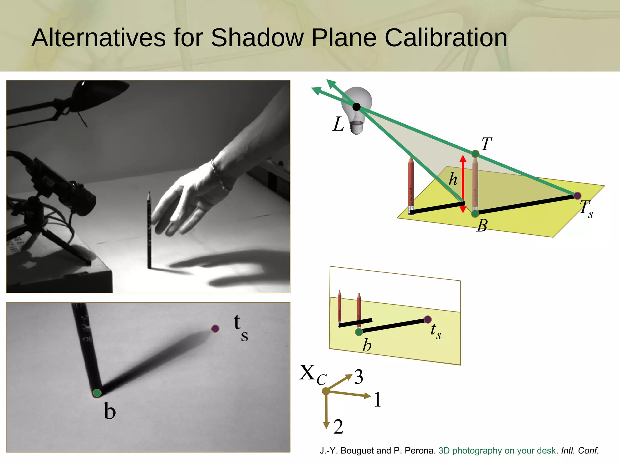
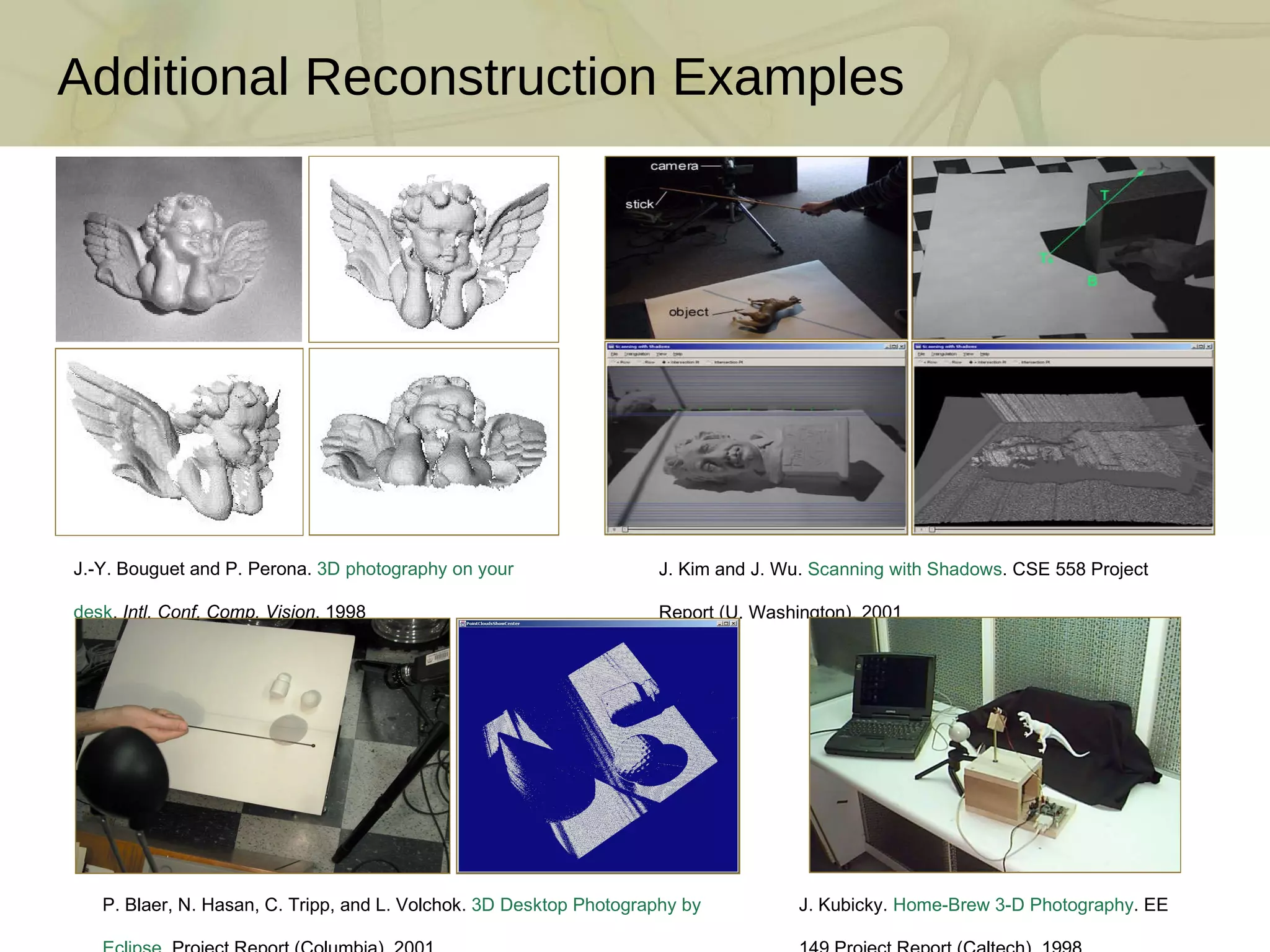
![3D Photography on Your Desk: Bouguet and Perona [ICCV 1998] J.-Y. Bouguet and P. Perona. 3D photography on your desk . Intl. Conf. Comp. Vision , 1998 DIY scanner using only a camera, a halogen lamp, and a stick Per-pixel depth by ray-plane triangulation Requires accurate camera and shadow plane calibration](https://image.slidesharecdn.com/swept-plane-090819160452-phpapp02/75/Build-Your-Own-3D-Scanner-3D-Scanning-with-Swept-Planes-3-2048.jpg)
![Assembling Your Own Scanner Parts: camera (QuickCam 9000), lamp, stick, two planar objects [~$100] Step 1: Build the calibration boards (include fiducials and chessboard) Step 2: Build the point light source (remove reflector and place in scene) Step 3: Arrange the camera, light source, and calibration boards](https://image.slidesharecdn.com/swept-plane-090819160452-phpapp02/75/Build-Your-Own-3D-Scanner-3D-Scanning-with-Swept-Planes-4-2048.jpg)
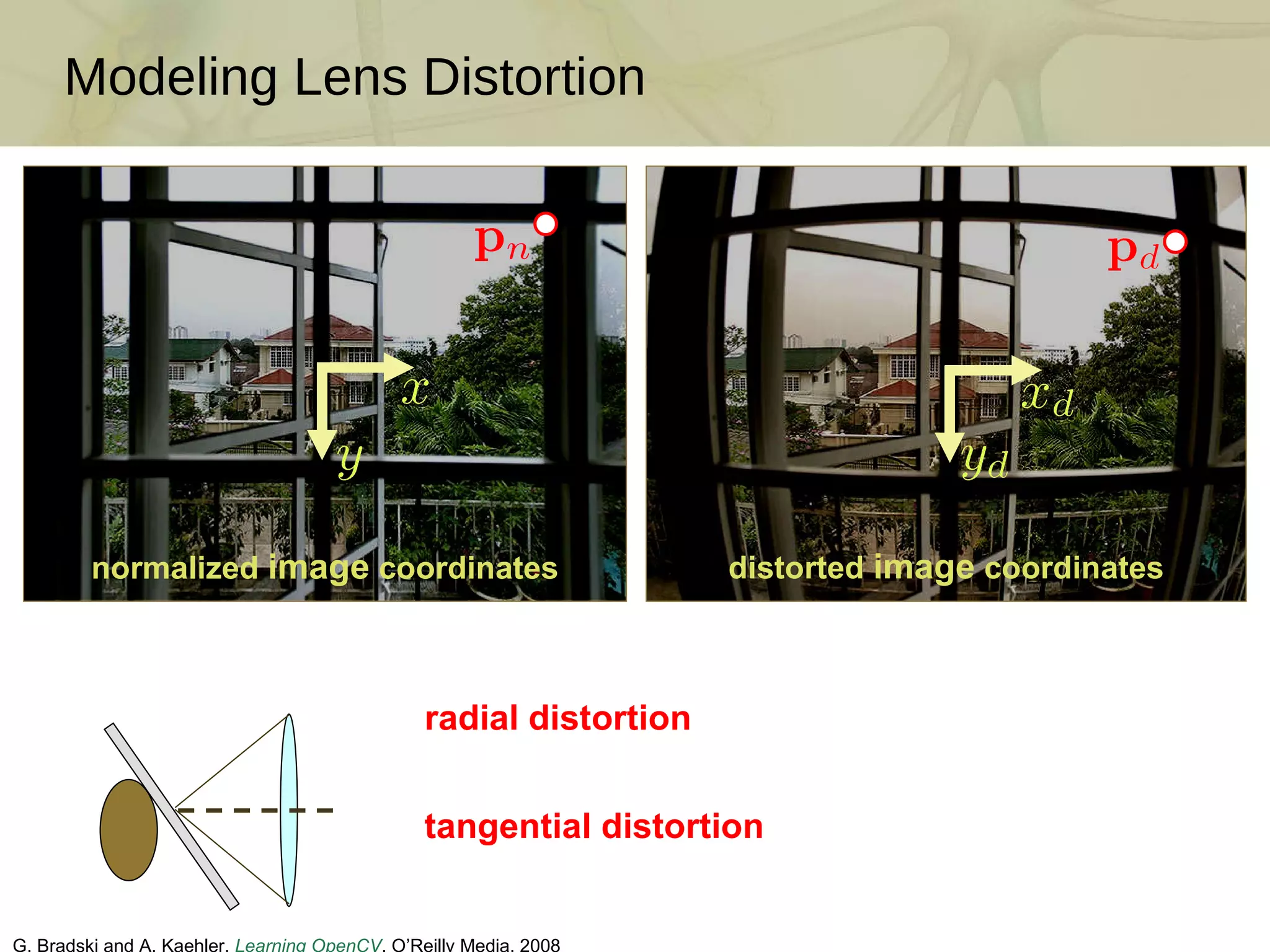
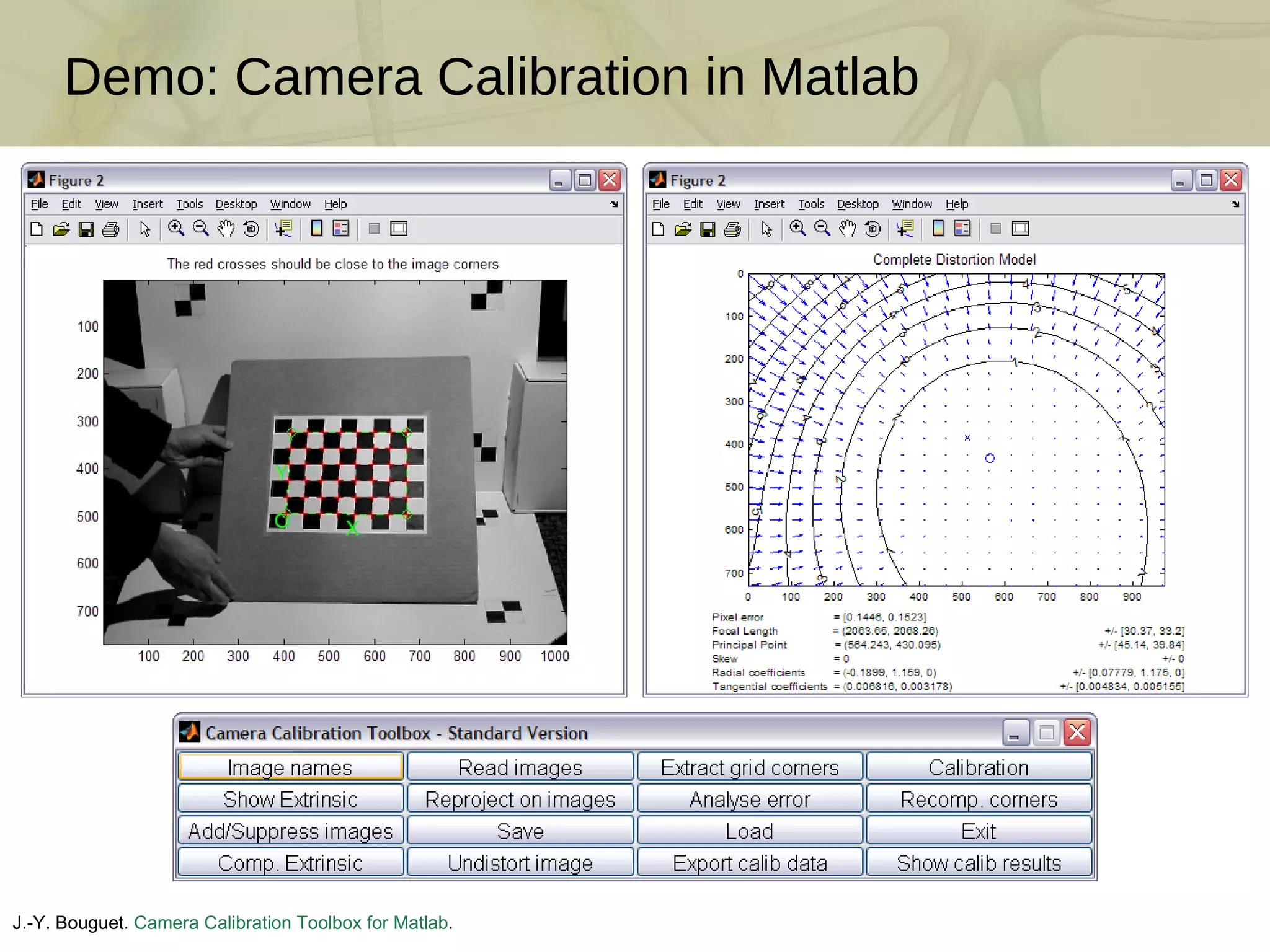
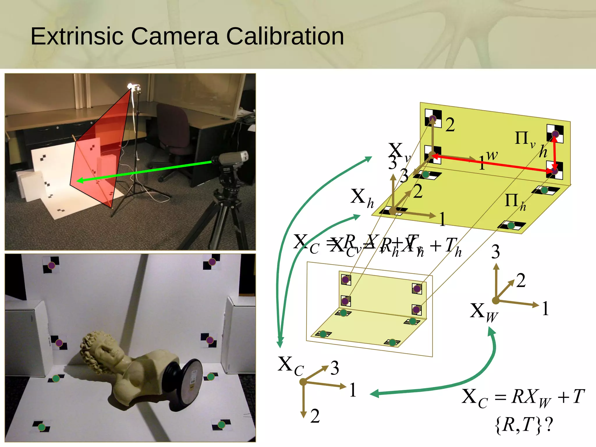
![Intrinsic Camera Calibration Camera Calibration Input How to estimate intrinsic parameters and distortion model? (unknowns: focal length, skew, scale, principal point, and distortion coeffs.) Popular solution: Observe a known calibration object (Zhang [2000]) Each 2D chessboard corner yields two constraints on the 6-11 unknowns But, must also find 6 extrinsic parameters per image (rotation/translation) Result: Two or more images of a chessboard are sufficient 1 1 1 1 1 1 2 2 2 2 2 2 3 3 3 3 4 4 4 5 5 6 6 7 Estimated Camera Lens Distortion Map camera coordinate system world coordinate system intrinsic parameters extrinsic parameters](https://image.slidesharecdn.com/swept-plane-090819160452-phpapp02/75/Build-Your-Own-3D-Scanner-3D-Scanning-with-Swept-Planes-12-2048.jpg)
![Visualizing Point Clouds: File Formats No standard file format to store point clouds Point = (x,y,z) plus (R,G,B) and/or (Nx,Ny,Nz) It is easy to create an ad-hoc file format Scene graph based file format: VRML International standard: ISO/IEC 14772-1:97 VRML’97 PointSet node includes coordinates (x,y,z) and optional colors (R,G,B), but no normals PointSet { coord Coordinate { point [ 0 -1 2, 1 0 0, -2 3 -1 ] } color Color { color [ 1 0 0, 0 1 0, 1 1 0 ] } }](https://image.slidesharecdn.com/swept-plane-090819160452-phpapp02/75/Build-Your-Own-3D-Scanner-3D-Scanning-with-Swept-Planes-24-2048.jpg)
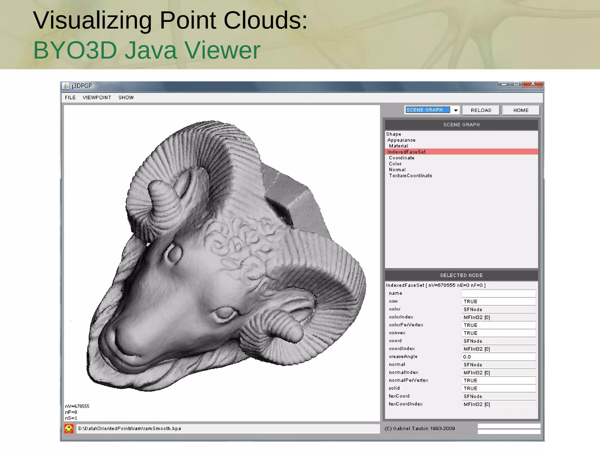
![Visualizing Point Clouds: File Formats IndexedFaceSet node designed to store a polygon mesh can be used to store point clouds with optional colors and/or normal vectors Store point coordinates as vertices Store point colors as colors per vertex Store point normal vectors as normals per vertex Degenerate polygon mesh with no faces is valid VRML syntax IndexedFaceSet { coord Coordinate { point [ 0 -1 2, 1 0 0, -2 3 -1 ] } colorPerVertex TRUE color Color { color [ 1 0 0, 0 1 0, 1 1 0 ] } normalPerVertex TRUE normal Normal { vector [ 1 0 0, 0 1 0, 0 0 1 ] } }](https://image.slidesharecdn.com/swept-plane-090819160452-phpapp02/75/Build-Your-Own-3D-Scanner-3D-Scanning-with-Swept-Planes-25-2048.jpg)
![Visualizing Point Clouds: Pointshop 3D [ Zwicker et al. 2002] M. Zwicker, M. Pauly, O. Knoll, M. Gross. Pointshop 3D: An Interactive System for Point-Based Surface Editing . ACM SIGGRAPH, 2002](https://image.slidesharecdn.com/swept-plane-090819160452-phpapp02/75/Build-Your-Own-3D-Scanner-3D-Scanning-with-Swept-Planes-27-2048.jpg)
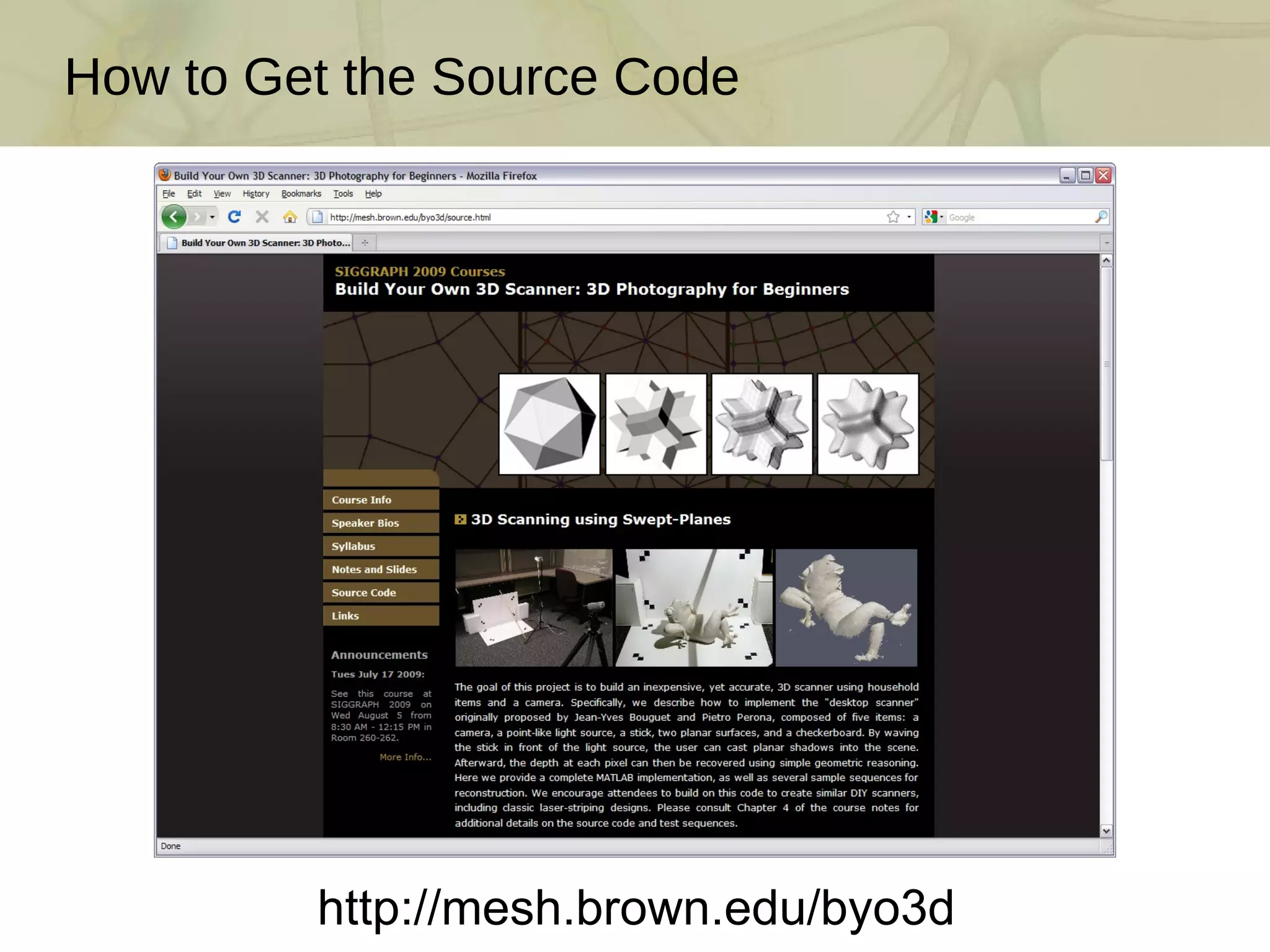
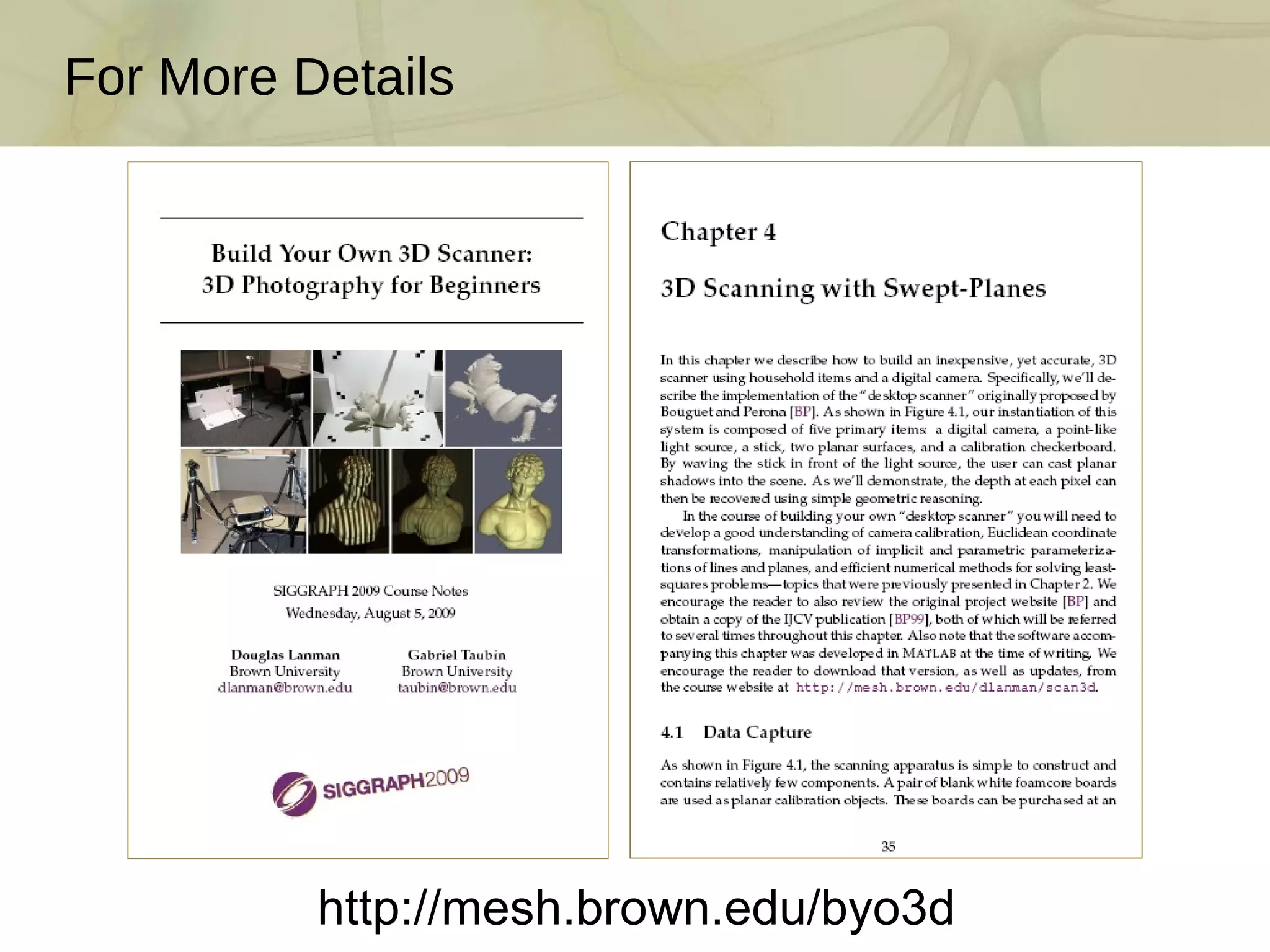

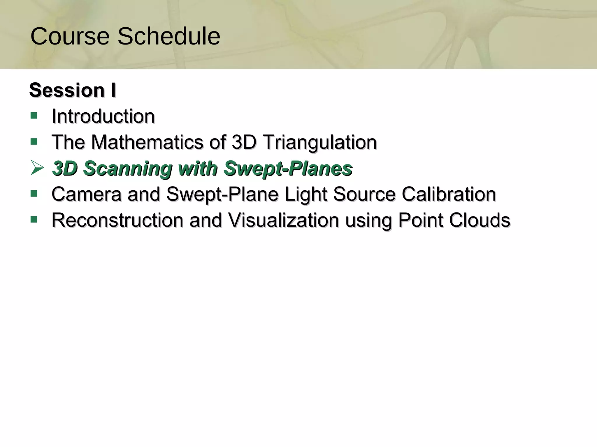
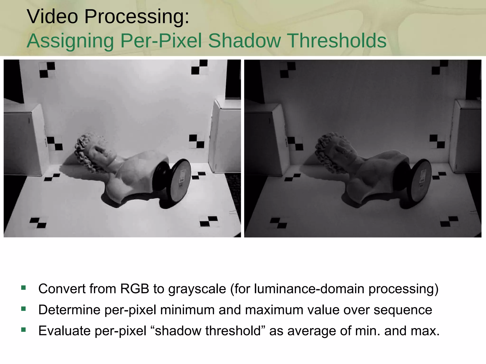
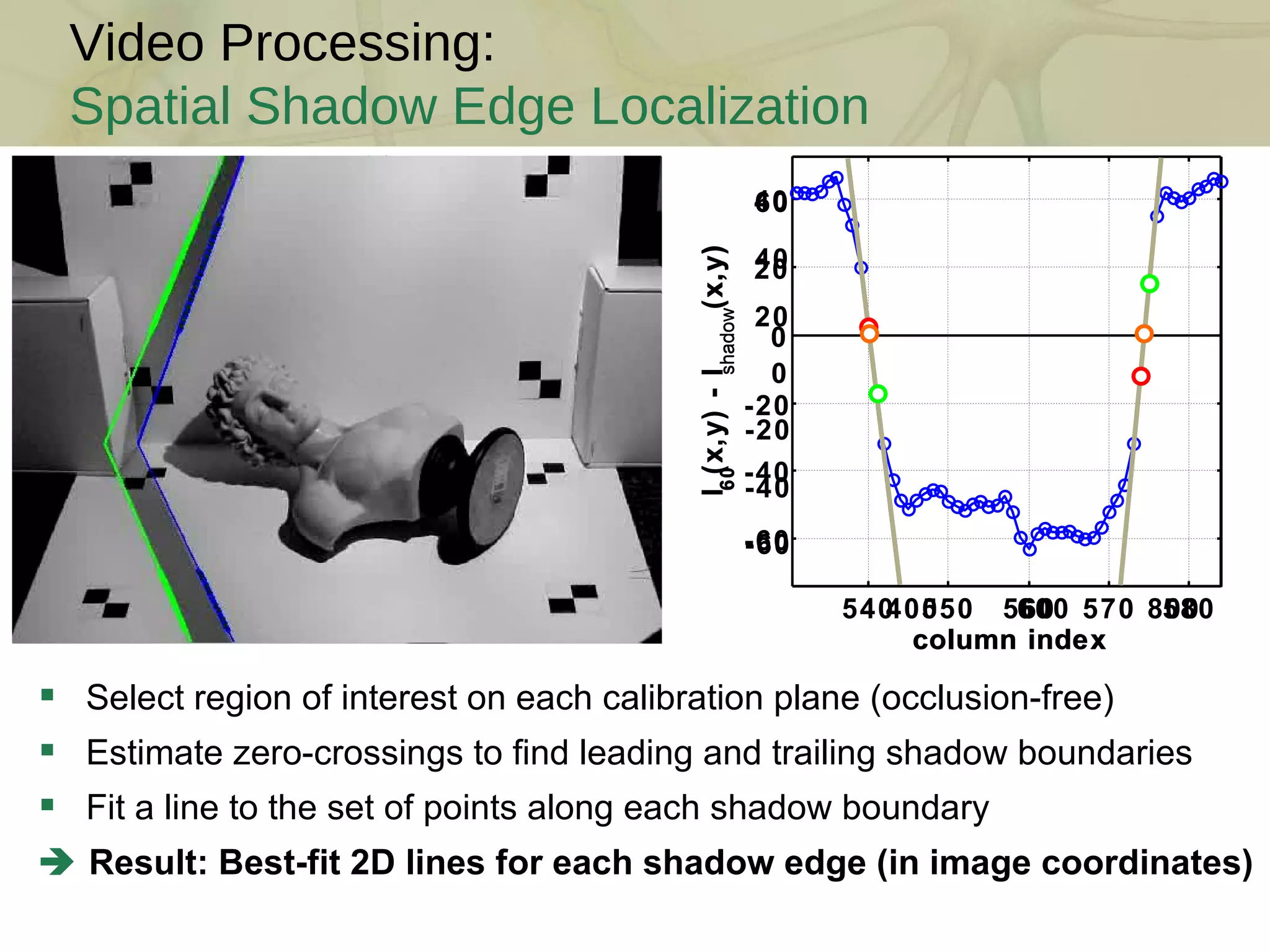
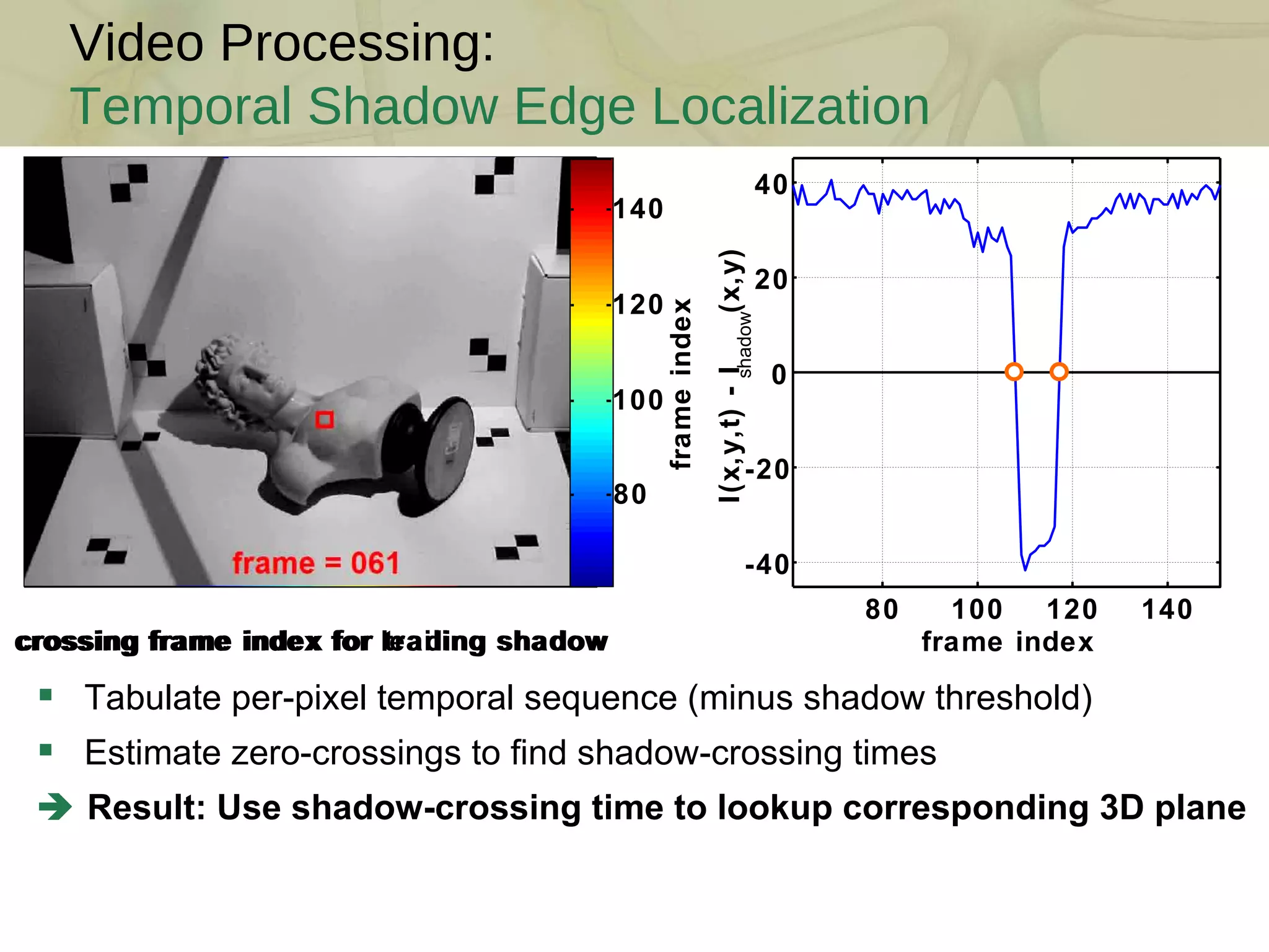
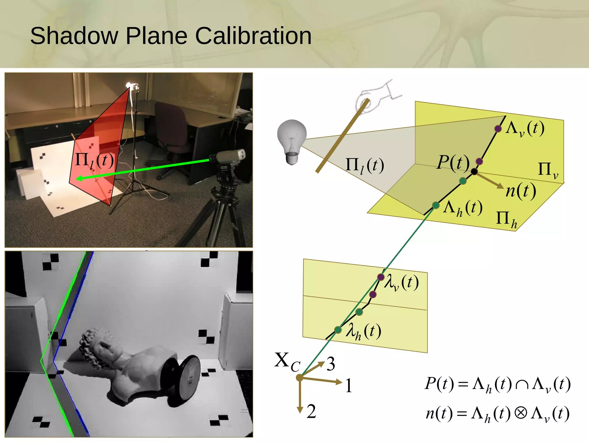
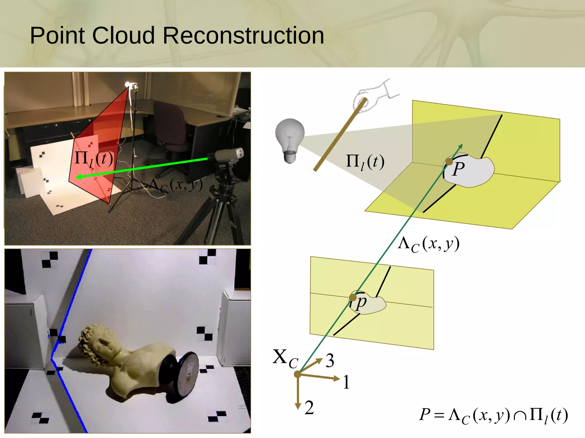
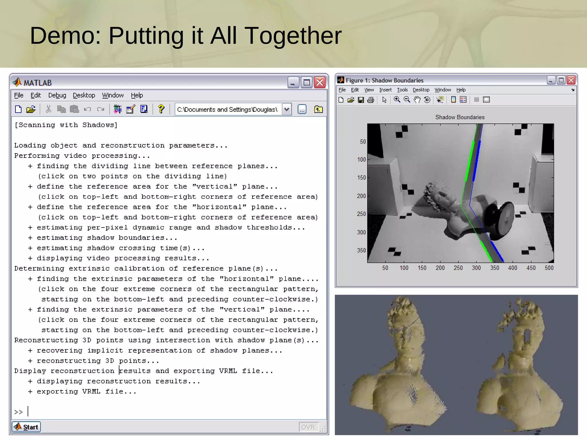
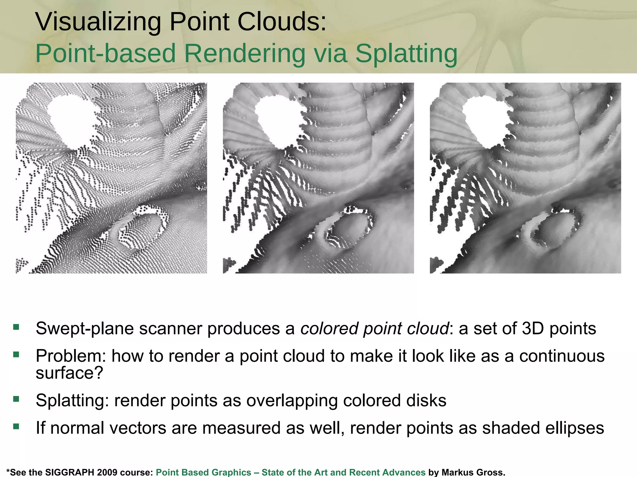
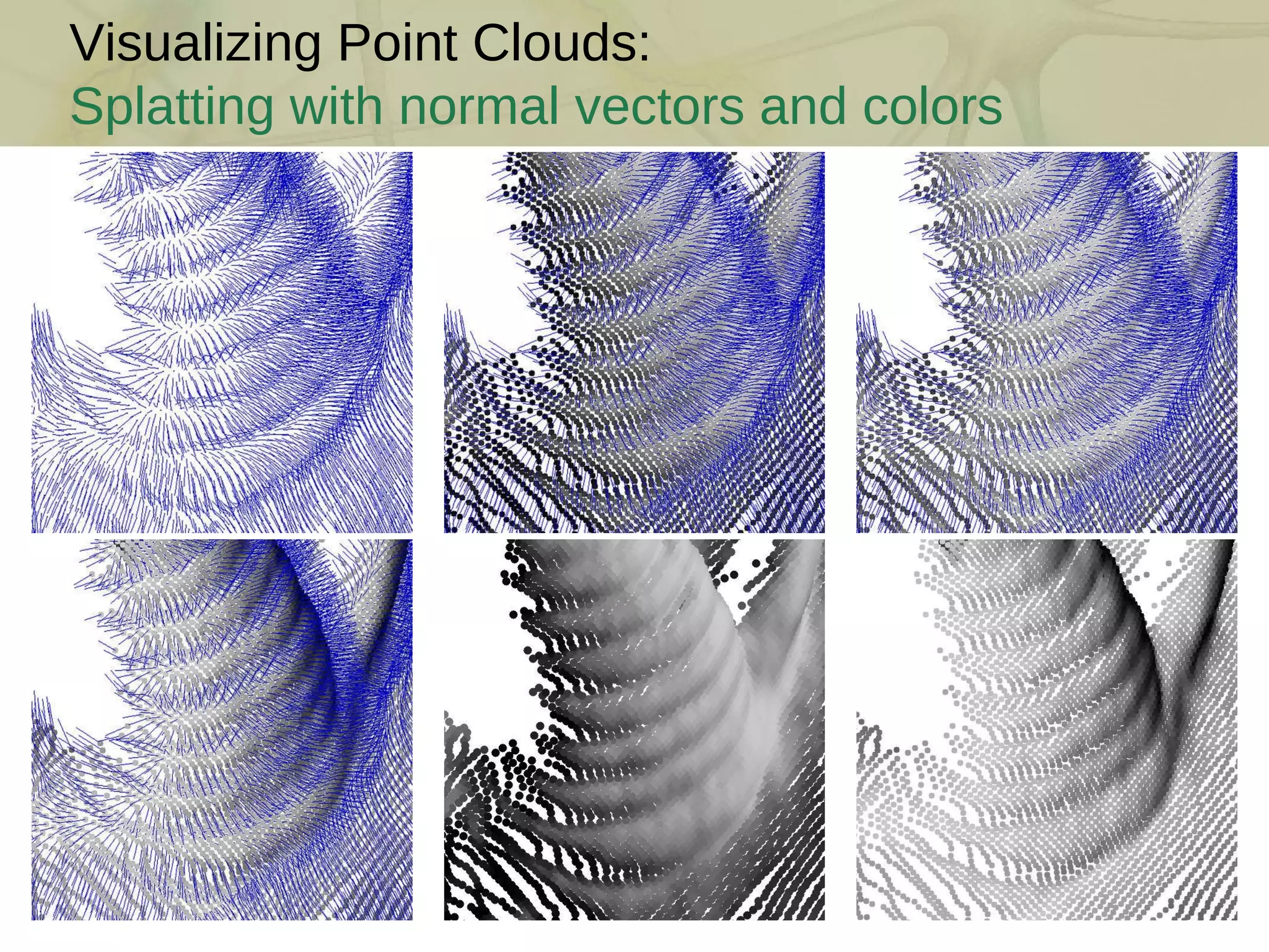
This document discusses the mathematics and techniques of 3D triangulation and scanning using swept-planes for camera and light source calibration. It covers the reconstruction and visualization of point clouds, along with detailed procedures for building DIY scanners, camera calibration, and visualizing point cloud data. Various examples and methodologies for shadow detection, edge localization, and surface rendering are presented, highlighting the tools and practices necessary for effectively capturing and displaying 3D information.


![[論文紹介] DPSNet: End-to-end Deep Plane Sweep Stereo](https://cdn.slidesharecdn.com/ss_thumbnails/20190212dpsnet-190830151623-thumbnail.jpg?width=640&height=640&fit=bounds)


