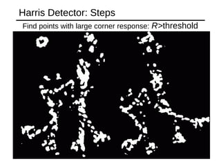
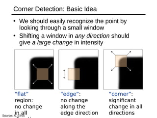
1
of
64
2
of
65
3-D Coordinate Spaces
Remember what we mean by a 3-D
coordinate space
x axis
y axis
z axis
P
y
z
x
Right-Hand
Reference System
3
of
65
4
of
65
Position of camera in space
5
of
65
The Up And Look Vectors
Up vector
Look vector
Position
Projection of up
vector
The look vector : indicates the direction in which the camera is
pointing
The up vector : determines how the camera is rotated
6
of
65
Rotations In 3-D
When we performed rotations in two
dimensions we only had the choice of
rotating about the z axis
In the case of three dimensions we have
more options
– Rotate about x – pitch
– Rotate about y – yaw
– Rotate about z - roll
7
of
64
Simple pinhole camera
A pinhole camera is a simple camera without a lens and with a single
small aperture. Light rays pass through the aperture and project an
inverted image on the opposite side of the camera. Think of the virtual
image plane as being in front of the camera and containing the upright
image of the scene.
8
of
65
9
of
65
-intrinsics,
-extrinsics,
-distortion coefficients.
Camera parameters include
10
of
65
Intrinsic Parameters
• principal point (u0,v0)
• scale factors (dx,dy)
• aspect ratio distortion factor 
• focal length f
• lens distortion factor 
(models radial lens distortion)
C
(u0,v0)
f
•intrinsic parameters are of the camera
device
11
of
65
Extrinsic Parameters
• translation parameters
t = [tx ty tz]
• rotation matrix
r11 r12 r13 0
r21 r22 r23 0
r31 r32 r33 0
0 0 0 1
R = Are there really
nine parameters?
extrinsic parameters are where the camera sits in the world
12
of
65
What Is Camera Calibration?
Geometric camera calibration
is the process of estimating intrinsic and/or extrinsic
parameters
You can use these parameters to
- correct for lens distortion,
- measure the size of an object in world units,
- determine the location of the camera in the
scene.
13
of
65
Camera Calibration Examples
14
of
65
15
of
65
The camera matrix does not account for lens
distortion because an ideal pinhole camera does
The Computer Vision Toolbox™ calibration
algorithm uses the camera model proposed by
Jean-Yves Bouguet
16
of
65
Scaling
• Scaling changes the size of an
object and involves two scale
factors, Sx and Sy for the x- and
y- coordinates respectively.
• Scales are about the origin.
• We can write the components:
p'x = sx • px
p'y = sy • py
or in matrix form:
P' = S • P
Scale matrix as:







y
x
s
s
S
0
0
P
P’
17
of
65
Translation
A translation moves all points in
an object along the same straight-
line path to new positions.
The path is represented by a
vector, called the translation or
shift vector.
We can write the components:
p'x = px + tx
p'y = py + ty
or in matrix form:
P' = P + T
tx
ty
x’
y’
x
y
tx
ty
= +
(2, 2)
= 6
=4
?
18
of
65
To estimate the camera parameters
You need to have 3-D world points and their
corresponding 2-D image points.
You can get these correspondences using multiple
images of a calibration pattern, such as a
checkerboard. Using the correspondences, you can
solve for the camera parameters.
19
of
65
calibration pattern
20
of
65
Chapter 14
Tut 14.1: Viewing Parameters
All viewing parameters
controlled by slider bars
21
of
65
Calibration Application
22
of
65
Calibration invers
After you calibrate a camera, to evaluate the
accuracy of the estimated parameters, you
can:
-Plot the relative locations of the camera and
the calibration pattern
-Calculate the re-projection errors.
-Calculate the parameter estimation errors.
-Use the Camera Calibrator to perform
camera calibration and evaluate the
accuracy of the estimated parameters.
23
of
65
Calibration Application
24
of
33
What Are Projections?
Our 3-D scenes are all specified in 3-D
world coordinates
To display these we need to generate a 2-D
image - project objects onto a picture
plane
So how do we figure out these projections?
Picture Plane
Objects in
World Space
25
of
33
Converting From 3-D To 2-D
Projection is just one part of the process of
converting from 3-D world coordinates to a
2-D image
Clip against
view volume
Project onto
projection
plane
Transform to
2-D device
coordinates
3-D world
coordinate
output
primitives
2-D device
coordinates
26
of
33
Types Of Projections
There are two broad classes of projection:
– Parallel: Typically used for architectural and
engineering drawings
– Perspective: Realistic looking and used in
computer graphics
Perspective ProjectionParallel Projection
27
of
65
Parallel Projection
28
of
65
Perspective Projection
29
of
33
Types Of Projections (cont…)
For anyone who did engineering or technical
drawing
30
of
33
Parallel Projections
Some examples of parallel projections
Orthographic Projection
Isometric Projection
31
of
33
Isometric Projections
Isometric projections have been used in
computer games from the very early days
of the industry up to today
Q*Bert Sim City Virtual Magic Kingdom
32
of
33
Perspective Projections
Perspective projections are much more
realistic than parallel projections
33
of
33
Perspective Projections
There are a number of different kinds of
perspective views
The most common are one-point and two
point perspectives
One Point Perspective
Projection
Two-Point
Perspective
Projection
34
of
65
Camera calibration revisited
What if world coordinates of reference 3D points are not
known?
We can use scene features such as vanishing points
Vanishing
point
Vanishing
line
Vanishing
point
Vertical vanishing
point
(at infinity)
35
of
65
Camera calibration revisited
36
of
65
1
2
3
4
5
5.3
2.8
3.3
Camera height
Measuring height
37
of
65
Measuring height without a ruler
38
of
65
Vanishing points
• All lines having the same direction share the same vanishing point
image plane
line in the scene
vanishing point v
camera
center
39
of
65
Computing vanishing points
• X∞ is a point at infinity, v is its projection: v = PX∞
• The vanishing point depends only on line direction
• All lines having direction D intersect at X∞
















1
30
20
10
tdz
tdy
tdx
tX
















t
dtz
dty
dtx
/1
/
/
/
30
20
10













0
3
2
1
d
d
d
X
v
X0 Xt
40
of
65
Calibration from vanishing points
Consider a scene with three orthogonal vanishing directions:
v2
v1
.
v3
.
ote: v1, v2 are finite vanishing points and v3 is an infinite vanishing point
41
of
65
Calibration from vanishing points
Consider a scene with three orthogonal vanishing directions:
v2
v1
.
v3
.
We can align the world coordinate system with these direction
42
of
65
Calibration from vanishing points
• p1 = P(1,0,0,0)T – the vanishing point in the x direction
• Similarly, p2 and p3 are the vanishing points in the y and z
directions
• p4 = P(0,0,0,1)T – projection of the origin of the world coordinate
system
• Problem: we can only know the four columns up to independent
scale factors, additional constraints needed to solve for them
 4321 ppppP 











****
****
****
43
of
65
Can solve for focal length, principal pointCannot recover focal
length, principal point is
the third vanishing point
1 2 3 4
1
2
3
4
Measurements on planes
Approach: unwarp then measure
What kind of warp is this?
Image rectification
To unwarp (rectify) an image
• solve for homography H given p and p′
– how many points are necessary to solve for H?
p
p′
46
of
65
47
of
65
Calibration from vanishing points:
Summary
• Solve for K (focal length, principal point) using three
orthogonal vanishing points
• Get rotation directly from vanishing points once calibration
matrix is known
• Advantages
• No need for calibration chart, 2D-3D correspondences
• Could be completely automatic
• Disadvantages
• Only applies to certain kinds of scenes
• Inaccuracies in computation of vanishing points
• Problems due to infinite vanishing points
48
of
65
Introduction to 3D Imaging
There are several ways to calculate
depth information using 2D camera
sensors or other optical sensing
technologies.
49
of
65
50
of
65
51
of
65
Human binocular vision
52
of
65
53
of
65
Double vision.
Vivek Nityananda, and Jenny C. A. Read J Exp Biol
2017;220:2502-2512
© 2017. Published by The Company of Biologists Ltd
54
of
65
stereo camera
• Stereo vision is the process of extracting 3-D
information from multiple 2-D views of a scene
• A stereo camera is a type of camera with two or
more image sensors. This allows the camera to
simulate human binocular vision and therefore
gives it the ability to perceive depth.
55
of
65
Two-view geometry
• In this case we have two camera views capture the
same scene from two different viewpoints
• from two images, we are interested in estimating the 3D
structure of the scene
56
of
65
Two-view geometry
• b is the baseline, or
distance between the two
cameras
• f is the focal length of a
camera
• XA is the X-axis of a
camera
• ZA is the optical axis of a
camera
• P is a real-world point
defined by the coordinates
X, Y, and Z
• uL is the projection of the
real-world point P in an
image acquired by the left
57
of
65
Two-view geometry
• Since the two cameras are separated by distance “b”, both
cameras view the same real-world point P in a different
location on the 2-dimensional images acquired.  
The X-coordinates of points uL and uR are given by
uL = f * X/Z
and
uR = f * (X-b)/Z
Distance between those two projected points is known
as “disparity” and we can use the disparity value to
calculate depth information, which is the distance
between real-world point “P” and the stereo vision
system. 
disparity  =   uL – uR   =  f *
b/z
58
of
65
Disparity
• Disparity refers to difference in pixel position between
two camera images. Assuming left image in stereo vision
camera has a pixel at position (1, 30) and the same pixel
is present at position (4, 30) in right image, the disparity
value or difference is (4 – 1) =3. Disparity value is
inversely proportional to depth as per the above formula.
59
of
65
Left image Right Image Right Image
Depth Image
60
of
65
Stereo Vision
depth map
Interest Points and Corners
An interest point may be composed of various types of corner,
edge, and maxima shapes. In general, a good interest point must
be easy to find and ideally fast to compute; it is hoped that the
interest point is at a good location to compute a feature descriptor.
The interest point is thus the qualifier or keypoint around which a
feature may be described
Example: estimating “fundamental
matrix” that corresponds two
views
Slide from Silvio Savarese
Example: structure from motion
interest points
• Note: “interest points” =
“keypoints”, also sometimes called
“features”
• Many applications
– tracking: which points are good to
track?
– recognition: find patches likely to tell
us something about object category
– 3D reconstruction: find
correspondences across different views
This class: interest points
• Suppose you have
to click on some
point, go away
and come back
after I deform the
image, and click
on the same
points again.
– Which points
would you choose?
original
deformed
Overview of Keypoint Matching
K. Grauman, B. Leibe
Af Bf
B1
B2
B3A1
A2 A3
Tffd BA ),(
1. Find a set of
distinctive key-
points
3. Extract and
normalize the
region content
2. Define a region
around each
keypoint
4. Compute a local
descriptor from the
normalized region
5. Match local
descriptors
Goals for Keypoints
Detect points that are repeatable and
distinctive
Invariant Local Features
Image content is transformed into local feature coordinates that are
invariant to translation, rotation, scale, and other imaging parameters
Features Descriptors
Feature extraction: Corners
9300 Harris Corners Pkwy, Charlotte, NC
Slides from Rick Szeliski, Svetlana Lazebnik, and Kristin Grauman
Many Existing Detectors
Available
K. Grauman, B. Leibe
Hessian & Harris [Beaudet ‘78], [Harris ‘88]
Laplacian, DoG [Lindeberg ‘98], [Lowe 1999]
Harris-/Hessian-Laplace [Mikolajczyk & Schmid
‘01]
Harris-/Hessian-Affine [Mikolajczyk & Schmid ‘04]
EBR and IBR [Tuytelaars & Van Gool ‘04]
MSER [Matas ‘02]
Salient Regions [Kadir & Brady ‘01]
Others…
Corner Detection: Basic Idea
• We should easily recognize the point by
looking through a small window
• Shifting a window in any direction should
give a large change in intensity
“edge”:
no change
along the
edge direction
“corner”:
significant
change in all
directions
“flat”
region:
no change
in allSource: A. Efros
Corner Detection: Mathematics
 
2
,
( , ) ( , ) ( , ) ( , )
x y
E u v w x y I x u y v I x y   
Change in appearance of window w(x,y)
for the shift [u,v]:
I(x, y)
E(u, v)
E(3,2)
w(x, y)
Corner Detection: Mathematics
 
2
,
( , ) ( , ) ( , ) ( , )
x y
E u v w x y I x u y v I x y   
I(x, y)
E(u, v)
E(0,0)
w(x, y)
Change in appearance of window w(x,y)
for the shift [u,v]:
Corner Detection: Mathematics
 
2
,
( , ) ( , ) ( , ) ( , )
x y
E u v w x y I x u y v I x y   
IntensityShifted
intensity
Window
function
orWindow function w(x,y) =
Gaussian1 in window, 0 outside
Source: R. Szeliski
Change in appearance of window w(x,y)
for the shift [u,v]:
Corner Detection: Mathematics
 
2
,
( , ) ( , ) ( , ) ( , )
x y
E u v w x y I x u y v I x y   
We want to find out how this function behaves for
small shifts
Change in appearance of window w(x,y)
for the shift [u,v]:
E(u, v)
Corner Detection: Mathematics
 
2
,
( , ) ( , ) ( , ) ( , )
x y
E u v w x y I x u y v I x y   
Local quadratic approximation of E(u,v) in the
neighborhood of (0,0) is given by the second-order
Taylor expansion:



















v
u
EE
EE
vu
E
E
vuEvuE
vvuv
uvuu
v
u
)0,0()0,0(
)0,0()0,0(
][
2
1
)0,0(
)0,0(
][)0,0(),(
We want to find out how this function behaves for
small shifts
Change in appearance of window w(x,y)
for the shift [u,v]:






 yyyx
yxxx
IIII
IIII
yxwM ),(
x
I
Ix



y
I
Iy



y
I
x
I
II yx





Corners as distinctive interest points
2 x 2 matrix of image derivatives (averaged in
neighborhood of a point).
Notation:
Corner response function
“Corner”
R > 0
“Edge”
R < 0
“Edge”
R < 0
“Flat”
region
|R| small
2
2121
2
)()(trace)det(   MMR
α: constant (0.04 to 0.06)
Harris corner detector
1) Compute M matrix for each image window to
get their cornerness scores.
2) Find points whose surrounding window gave
large corner response (f> threshold)
3) Take the points of local maxima, i.e., perform
non-maximum suppression
C.Harris and M.Stephens. “A Combined Corner and Edge Detector.”
Proceedings of the 4th Alvey Vision Conference: pages 147—151, 1988. 
Harris Detector [Harris88]
• Second moment
matrix









)()(
)()(
)(),( 2
2
DyDyx
DyxDx
IDI
III
III
g



83
1. Image
derivatives
2. Square of
derivatives
3. Gaussian
filter g(I)
Ix Iy
Ix
2 Iy
2
IxIy
g(Ix
2
) g(Iy
2
) g(IxIy)
222222
)]()([)]([)()( yxyxyx IgIgIIgIgIg  
 ])),([trace()],(det[ 2
DIDIhar 
4. Cornerness function – both eigenvalues are strong
har5. Non-maxima suppression
1 2
1 2
det
trace
M
M
 
 

 
(optionally, blur first)
Harris Detector: Steps
Compute corner response R
Harris Detector: Steps
Find points with large corner response: R>threshold
Harris Detector: Steps
Take only the points of local maxima of R
Harris Detector: Steps
89
of
65
Epipolar geometry
• the 3D points P, C1,C2  and the projected
points p1, p2 are all located within one common plane
• This common plane denoted π is known as
the epipolar plane
90
of
65
Epipolar geometry
• The epipolar plane is the plane defined by a 3D
point and the two cameras centers.
• The epipolar line is the line determined by the
intersection of the image plane with the epipolar
plane.
• The baseline is the line going through the two
cameras centers.
• The epipole is the image-point determined by the
intersection of the image plane with the baseline.
• the epipole corresponds to the projection of the
first camera center (say C1) onto the second
image plane (say I2), or vice versa.
91
of
65
Epipolar Lines – Example
92
of
65
What is Mosaic and Mosaicing?
• “Mosaic“ originates from an old Italian word
“mosaico” which means a picture or pattern
produced by arranging together small pieces of
stone, tile, glass, etc.
• Mosaicing is the process of assembling a series of
images and joining them together to form a
continuous seamless photographic representation
of the image surface.
• The result is an image with a field of view greater
than that of a single image
93
of
65
Why We Need Image
Mosaicing?
Image mosaicing not only allow you to create a large
field of view using normal camera, the result image
can also be used for texture mapping of a 3D
environment such that users can view the
surrounding scene with real images.
94
of
65
image mosaicing:
Basically there are two main algorithms of image mosaicin
2)Bi-directional Scanning
1)Unidirectional Scanning
95
of
65
Richard Szeliski Image Stitching 95
RANSAC motion model
96
of
65
Richard Szeliski Image Stitching 96
RANSAC motion model
97
of
65
Richard Szeliski Image Stitching 97
RANSAC motion model

Saad alsheekh multi view

  • 1.
  • 2.
    2 of 65 3-D Coordinate Spaces Rememberwhat we mean by a 3-D coordinate space x axis y axis z axis P y z x Right-Hand Reference System
  • 3.
  • 4.
  • 5.
    5 of 65 The Up AndLook Vectors Up vector Look vector Position Projection of up vector The look vector : indicates the direction in which the camera is pointing The up vector : determines how the camera is rotated
  • 6.
    6 of 65 Rotations In 3-D Whenwe performed rotations in two dimensions we only had the choice of rotating about the z axis In the case of three dimensions we have more options – Rotate about x – pitch – Rotate about y – yaw – Rotate about z - roll
  • 7.
    7 of 64 Simple pinhole camera Apinhole camera is a simple camera without a lens and with a single small aperture. Light rays pass through the aperture and project an inverted image on the opposite side of the camera. Think of the virtual image plane as being in front of the camera and containing the upright image of the scene.
  • 8.
  • 9.
  • 10.
    10 of 65 Intrinsic Parameters • principalpoint (u0,v0) • scale factors (dx,dy) • aspect ratio distortion factor  • focal length f • lens distortion factor  (models radial lens distortion) C (u0,v0) f •intrinsic parameters are of the camera device
  • 11.
    11 of 65 Extrinsic Parameters • translationparameters t = [tx ty tz] • rotation matrix r11 r12 r13 0 r21 r22 r23 0 r31 r32 r33 0 0 0 0 1 R = Are there really nine parameters? extrinsic parameters are where the camera sits in the world
  • 12.
    12 of 65 What Is CameraCalibration? Geometric camera calibration is the process of estimating intrinsic and/or extrinsic parameters You can use these parameters to - correct for lens distortion, - measure the size of an object in world units, - determine the location of the camera in the scene.
  • 13.
  • 14.
  • 15.
    15 of 65 The camera matrixdoes not account for lens distortion because an ideal pinhole camera does The Computer Vision Toolbox™ calibration algorithm uses the camera model proposed by Jean-Yves Bouguet
  • 16.
    16 of 65 Scaling • Scaling changesthe size of an object and involves two scale factors, Sx and Sy for the x- and y- coordinates respectively. • Scales are about the origin. • We can write the components: p'x = sx • px p'y = sy • py or in matrix form: P' = S • P Scale matrix as:        y x s s S 0 0 P P’
  • 17.
    17 of 65 Translation A translation movesall points in an object along the same straight- line path to new positions. The path is represented by a vector, called the translation or shift vector. We can write the components: p'x = px + tx p'y = py + ty or in matrix form: P' = P + T tx ty x’ y’ x y tx ty = + (2, 2) = 6 =4 ?
  • 18.
    18 of 65 To estimate thecamera parameters You need to have 3-D world points and their corresponding 2-D image points. You can get these correspondences using multiple images of a calibration pattern, such as a checkerboard. Using the correspondences, you can solve for the camera parameters.
  • 19.
  • 20.
    20 of 65 Chapter 14 Tut 14.1:Viewing Parameters All viewing parameters controlled by slider bars
  • 21.
  • 22.
    22 of 65 Calibration invers After youcalibrate a camera, to evaluate the accuracy of the estimated parameters, you can: -Plot the relative locations of the camera and the calibration pattern -Calculate the re-projection errors. -Calculate the parameter estimation errors. -Use the Camera Calibrator to perform camera calibration and evaluate the accuracy of the estimated parameters.
  • 23.
  • 24.
    24 of 33 What Are Projections? Our3-D scenes are all specified in 3-D world coordinates To display these we need to generate a 2-D image - project objects onto a picture plane So how do we figure out these projections? Picture Plane Objects in World Space
  • 25.
    25 of 33 Converting From 3-DTo 2-D Projection is just one part of the process of converting from 3-D world coordinates to a 2-D image Clip against view volume Project onto projection plane Transform to 2-D device coordinates 3-D world coordinate output primitives 2-D device coordinates
  • 26.
    26 of 33 Types Of Projections Thereare two broad classes of projection: – Parallel: Typically used for architectural and engineering drawings – Perspective: Realistic looking and used in computer graphics Perspective ProjectionParallel Projection
  • 27.
  • 28.
  • 29.
    29 of 33 Types Of Projections(cont…) For anyone who did engineering or technical drawing
  • 30.
    30 of 33 Parallel Projections Some examplesof parallel projections Orthographic Projection Isometric Projection
  • 31.
    31 of 33 Isometric Projections Isometric projectionshave been used in computer games from the very early days of the industry up to today Q*Bert Sim City Virtual Magic Kingdom
  • 32.
    32 of 33 Perspective Projections Perspective projectionsare much more realistic than parallel projections
  • 33.
    33 of 33 Perspective Projections There area number of different kinds of perspective views The most common are one-point and two point perspectives One Point Perspective Projection Two-Point Perspective Projection
  • 34.
    34 of 65 Camera calibration revisited Whatif world coordinates of reference 3D points are not known? We can use scene features such as vanishing points Vanishing point Vanishing line Vanishing point Vertical vanishing point (at infinity)
  • 35.
  • 36.
  • 37.
  • 38.
    38 of 65 Vanishing points • Alllines having the same direction share the same vanishing point image plane line in the scene vanishing point v camera center
  • 39.
    39 of 65 Computing vanishing points •X∞ is a point at infinity, v is its projection: v = PX∞ • The vanishing point depends only on line direction • All lines having direction D intersect at X∞                 1 30 20 10 tdz tdy tdx tX                 t dtz dty dtx /1 / / / 30 20 10              0 3 2 1 d d d X v X0 Xt
  • 40.
    40 of 65 Calibration from vanishingpoints Consider a scene with three orthogonal vanishing directions: v2 v1 . v3 . ote: v1, v2 are finite vanishing points and v3 is an infinite vanishing point
  • 41.
    41 of 65 Calibration from vanishingpoints Consider a scene with three orthogonal vanishing directions: v2 v1 . v3 . We can align the world coordinate system with these direction
  • 42.
    42 of 65 Calibration from vanishingpoints • p1 = P(1,0,0,0)T – the vanishing point in the x direction • Similarly, p2 and p3 are the vanishing points in the y and z directions • p4 = P(0,0,0,1)T – projection of the origin of the world coordinate system • Problem: we can only know the four columns up to independent scale factors, additional constraints needed to solve for them  4321 ppppP             **** **** ****
  • 43.
    43 of 65 Can solve forfocal length, principal pointCannot recover focal length, principal point is the third vanishing point
  • 44.
    1 2 34 1 2 3 4 Measurements on planes Approach: unwarp then measure What kind of warp is this?
  • 45.
    Image rectification To unwarp(rectify) an image • solve for homography H given p and p′ – how many points are necessary to solve for H? p p′
  • 46.
  • 47.
    47 of 65 Calibration from vanishingpoints: Summary • Solve for K (focal length, principal point) using three orthogonal vanishing points • Get rotation directly from vanishing points once calibration matrix is known • Advantages • No need for calibration chart, 2D-3D correspondences • Could be completely automatic • Disadvantages • Only applies to certain kinds of scenes • Inaccuracies in computation of vanishing points • Problems due to infinite vanishing points
  • 48.
    48 of 65 Introduction to 3DImaging There are several ways to calculate depth information using 2D camera sensors or other optical sensing technologies.
  • 49.
  • 50.
  • 51.
  • 52.
  • 53.
    53 of 65 Double vision. Vivek Nityananda,and Jenny C. A. Read J Exp Biol 2017;220:2502-2512 © 2017. Published by The Company of Biologists Ltd
  • 54.
    54 of 65 stereo camera • Stereovision is the process of extracting 3-D information from multiple 2-D views of a scene • A stereo camera is a type of camera with two or more image sensors. This allows the camera to simulate human binocular vision and therefore gives it the ability to perceive depth.
  • 55.
    55 of 65 Two-view geometry • Inthis case we have two camera views capture the same scene from two different viewpoints • from two images, we are interested in estimating the 3D structure of the scene
  • 56.
    56 of 65 Two-view geometry • bis the baseline, or distance between the two cameras • f is the focal length of a camera • XA is the X-axis of a camera • ZA is the optical axis of a camera • P is a real-world point defined by the coordinates X, Y, and Z • uL is the projection of the real-world point P in an image acquired by the left
  • 57.
    57 of 65 Two-view geometry • Sincethe two cameras are separated by distance “b”, both cameras view the same real-world point P in a different location on the 2-dimensional images acquired.   The X-coordinates of points uL and uR are given by uL = f * X/Z and uR = f * (X-b)/Z Distance between those two projected points is known as “disparity” and we can use the disparity value to calculate depth information, which is the distance between real-world point “P” and the stereo vision system.  disparity  =   uL – uR   =  f * b/z
  • 58.
    58 of 65 Disparity • Disparity refersto difference in pixel position between two camera images. Assuming left image in stereo vision camera has a pixel at position (1, 30) and the same pixel is present at position (4, 30) in right image, the disparity value or difference is (4 – 1) =3. Disparity value is inversely proportional to depth as per the above formula.
  • 59.
    59 of 65 Left image RightImage Right Image Depth Image
  • 60.
  • 61.
    Interest Points andCorners An interest point may be composed of various types of corner, edge, and maxima shapes. In general, a good interest point must be easy to find and ideally fast to compute; it is hoped that the interest point is at a good location to compute a feature descriptor. The interest point is thus the qualifier or keypoint around which a feature may be described
  • 62.
    Example: estimating “fundamental matrix”that corresponds two views Slide from Silvio Savarese
  • 63.
  • 64.
    interest points • Note:“interest points” = “keypoints”, also sometimes called “features” • Many applications – tracking: which points are good to track? – recognition: find patches likely to tell us something about object category – 3D reconstruction: find correspondences across different views
  • 65.
    This class: interestpoints • Suppose you have to click on some point, go away and come back after I deform the image, and click on the same points again. – Which points would you choose? original deformed
  • 66.
    Overview of KeypointMatching K. Grauman, B. Leibe Af Bf B1 B2 B3A1 A2 A3 Tffd BA ),( 1. Find a set of distinctive key- points 3. Extract and normalize the region content 2. Define a region around each keypoint 4. Compute a local descriptor from the normalized region 5. Match local descriptors
  • 67.
    Goals for Keypoints Detectpoints that are repeatable and distinctive
  • 68.
    Invariant Local Features Imagecontent is transformed into local feature coordinates that are invariant to translation, rotation, scale, and other imaging parameters Features Descriptors
  • 69.
    Feature extraction: Corners 9300Harris Corners Pkwy, Charlotte, NC Slides from Rick Szeliski, Svetlana Lazebnik, and Kristin Grauman
  • 70.
    Many Existing Detectors Available K.Grauman, B. Leibe Hessian & Harris [Beaudet ‘78], [Harris ‘88] Laplacian, DoG [Lindeberg ‘98], [Lowe 1999] Harris-/Hessian-Laplace [Mikolajczyk & Schmid ‘01] Harris-/Hessian-Affine [Mikolajczyk & Schmid ‘04] EBR and IBR [Tuytelaars & Van Gool ‘04] MSER [Matas ‘02] Salient Regions [Kadir & Brady ‘01] Others…
  • 71.
    Corner Detection: BasicIdea • We should easily recognize the point by looking through a small window • Shifting a window in any direction should give a large change in intensity “edge”: no change along the edge direction “corner”: significant change in all directions “flat” region: no change in allSource: A. Efros
  • 72.
    Corner Detection: Mathematics  2 , ( , ) ( , ) ( , ) ( , ) x y E u v w x y I x u y v I x y    Change in appearance of window w(x,y) for the shift [u,v]: I(x, y) E(u, v) E(3,2) w(x, y)
  • 73.
    Corner Detection: Mathematics  2 , ( , ) ( , ) ( , ) ( , ) x y E u v w x y I x u y v I x y    I(x, y) E(u, v) E(0,0) w(x, y) Change in appearance of window w(x,y) for the shift [u,v]:
  • 74.
    Corner Detection: Mathematics  2 , ( , ) ( , ) ( , ) ( , ) x y E u v w x y I x u y v I x y    IntensityShifted intensity Window function orWindow function w(x,y) = Gaussian1 in window, 0 outside Source: R. Szeliski Change in appearance of window w(x,y) for the shift [u,v]:
  • 75.
    Corner Detection: Mathematics  2 , ( , ) ( , ) ( , ) ( , ) x y E u v w x y I x u y v I x y    We want to find out how this function behaves for small shifts Change in appearance of window w(x,y) for the shift [u,v]: E(u, v)
  • 76.
    Corner Detection: Mathematics  2 , ( , ) ( , ) ( , ) ( , ) x y E u v w x y I x u y v I x y    Local quadratic approximation of E(u,v) in the neighborhood of (0,0) is given by the second-order Taylor expansion:                    v u EE EE vu E E vuEvuE vvuv uvuu v u )0,0()0,0( )0,0()0,0( ][ 2 1 )0,0( )0,0( ][)0,0(),( We want to find out how this function behaves for small shifts Change in appearance of window w(x,y) for the shift [u,v]:
  • 77.
           yyyx yxxx IIII IIII yxwM ),( x I Ix    y I Iy    y I x I IIyx      Corners as distinctive interest points 2 x 2 matrix of image derivatives (averaged in neighborhood of a point). Notation:
  • 78.
    Corner response function “Corner” R> 0 “Edge” R < 0 “Edge” R < 0 “Flat” region |R| small 2 2121 2 )()(trace)det(   MMR α: constant (0.04 to 0.06)
  • 79.
    Harris corner detector 1)Compute M matrix for each image window to get their cornerness scores. 2) Find points whose surrounding window gave large corner response (f> threshold) 3) Take the points of local maxima, i.e., perform non-maximum suppression C.Harris and M.Stephens. “A Combined Corner and Edge Detector.” Proceedings of the 4th Alvey Vision Conference: pages 147—151, 1988. 
  • 80.
    Harris Detector [Harris88] •Second moment matrix          )()( )()( )(),( 2 2 DyDyx DyxDx IDI III III g    83 1. Image derivatives 2. Square of derivatives 3. Gaussian filter g(I) Ix Iy Ix 2 Iy 2 IxIy g(Ix 2 ) g(Iy 2 ) g(IxIy) 222222 )]()([)]([)()( yxyxyx IgIgIIgIgIg    ])),([trace()],(det[ 2 DIDIhar  4. Cornerness function – both eigenvalues are strong har5. Non-maxima suppression 1 2 1 2 det trace M M        (optionally, blur first)
  • 81.
  • 82.
  • 83.
    Harris Detector: Steps Findpoints with large corner response: R>threshold
  • 84.
    Harris Detector: Steps Takeonly the points of local maxima of R
  • 85.
  • 86.
    89 of 65 Epipolar geometry • the3D points P, C1,C2  and the projected points p1, p2 are all located within one common plane • This common plane denoted π is known as the epipolar plane
  • 87.
    90 of 65 Epipolar geometry • Theepipolar plane is the plane defined by a 3D point and the two cameras centers. • The epipolar line is the line determined by the intersection of the image plane with the epipolar plane. • The baseline is the line going through the two cameras centers. • The epipole is the image-point determined by the intersection of the image plane with the baseline. • the epipole corresponds to the projection of the first camera center (say C1) onto the second image plane (say I2), or vice versa.
  • 88.
  • 89.
    92 of 65 What is Mosaicand Mosaicing? • “Mosaic“ originates from an old Italian word “mosaico” which means a picture or pattern produced by arranging together small pieces of stone, tile, glass, etc. • Mosaicing is the process of assembling a series of images and joining them together to form a continuous seamless photographic representation of the image surface. • The result is an image with a field of view greater than that of a single image
  • 90.
    93 of 65 Why We NeedImage Mosaicing? Image mosaicing not only allow you to create a large field of view using normal camera, the result image can also be used for texture mapping of a 3D environment such that users can view the surrounding scene with real images.
  • 91.
    94 of 65 image mosaicing: Basically thereare two main algorithms of image mosaicin 2)Bi-directional Scanning 1)Unidirectional Scanning
  • 92.
    95 of 65 Richard Szeliski ImageStitching 95 RANSAC motion model
  • 93.
    96 of 65 Richard Szeliski ImageStitching 96 RANSAC motion model
  • 94.
    97 of 65 Richard Szeliski ImageStitching 97 RANSAC motion model