Downloaded 808 times
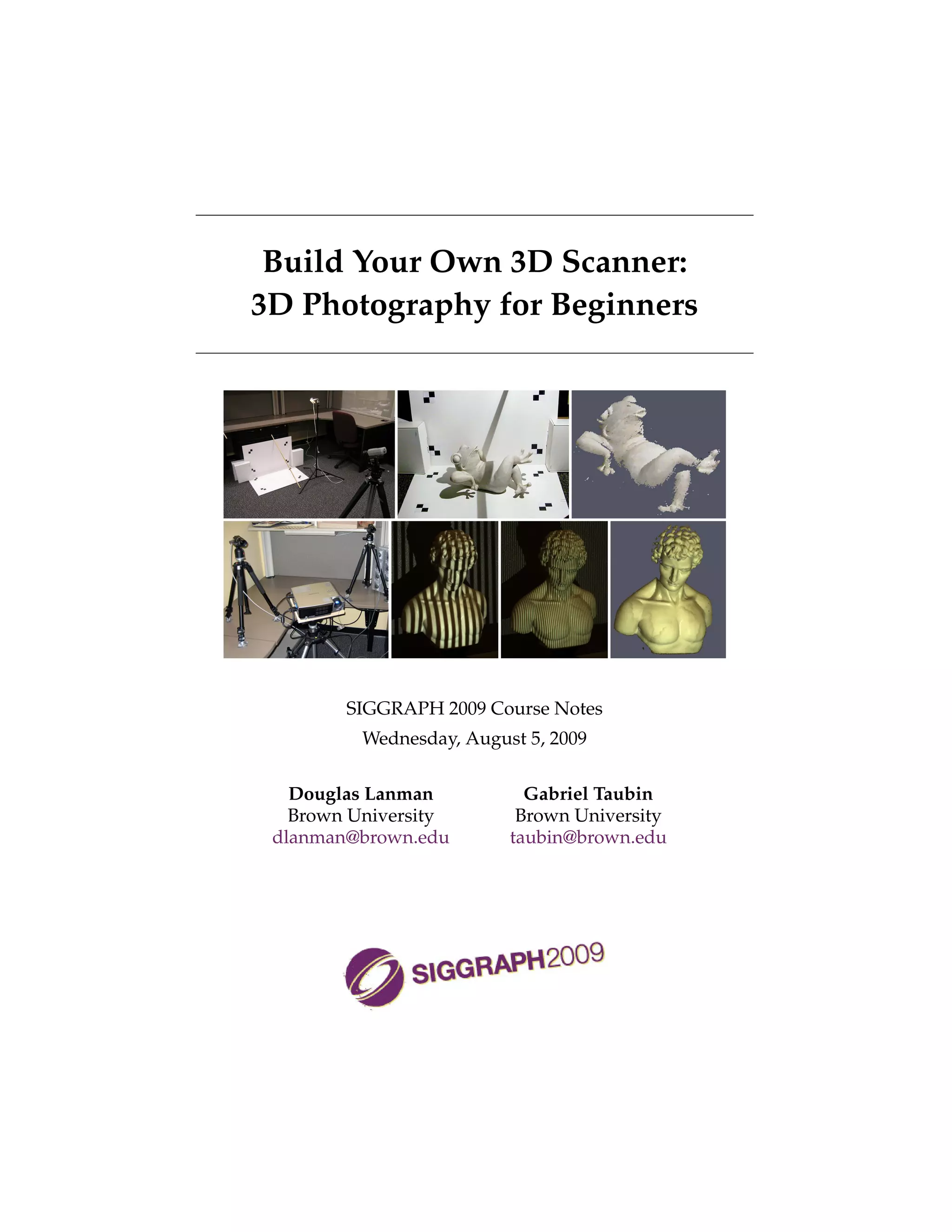


![Introduction to 3D Photography 3D Scanning Technology
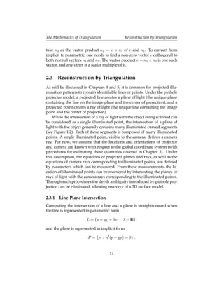
1.1 3D Scanning Technology
Metrology is an ancient and diverse field, bridging the gap between mathe-
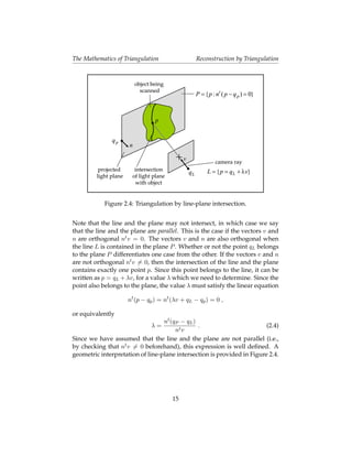
matics and engineering. Efforts at measurement standardization were first
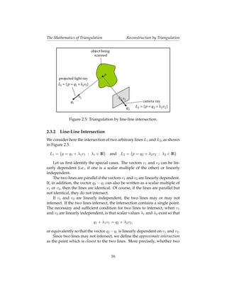
undertaken by the Indus Valley Civilization as early as 2600–1900 BCE.
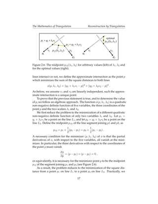
Even with only crude units, such as the length of human appendages, the
development of geometry revolutionized the ability to measure distance
accurately. Around 240 BCE, Eratosthenes estimated the circumference of
the Earth from knowledge of the elevation angle of the Sun during the sum-
mer solstice in Alexandria and Syene. Mathematics and standardization
efforts continued to mature through the Renaissance (1300–1600 CE) and
into the Scientific Revolution (1550–1700 CE). However, it was the Indus-
trial Revolution (1750–1850 CE) which drove metrology to the forefront.
As automatized methods of mass production became commonplace, ad-
vanced measurement technologies ensured interchangeable parts were just
that–accurate copies of the original.
Through these historical developments, measurement tools varied with
mathematical knowledge and practical needs. Early methods required di-
rect contact with a surface (e.g., callipers and rulers). The pantograph, in-
vented in 1603 by Christoph Scheiner, uses a special mechanical linkage
so movement of a stylus (in contact with the surface) can be precisely du-
plicated by a drawing pen. The modern coordinate measuring machine
(CMM) functions in much the same manner, recording the displacement of
a probe tip as it slides across a solid surface (see Figure 1.1). While effective,
such contact-based methods can harm fragile objects and require long pe-
riods of time to build an accurate 3D model. Non-contact scanners address
these limitations by observing, and possibly controlling, the interaction of
light with the object.
1.1.1 Passive Methods
Non-contact optical scanners can be categorized by the degree to which
controlled illumination is required. Passive scanners do not require di-
rect control of any illumination source, instead relying entirely on ambi-
ent light. Stereoscopic imaging is one of the most widely used passive 3D
imaging systems, both in biology and engineering. Mirroring the human
visual system, stereoscopy estimates the position of a 3D scene point by
triangulation [LN04]; first, the 2D projection of a given point is identified
in each camera. Using known calibration objects, the imaging properties
of each camera are estimated, ultimately allowing a single 3D line to be
2](https://image.slidesharecdn.com/byo3d-090819162830-phpapp01/85/Build-Your-Own-3D-Scanner-Course-Notes-9-320.jpg)
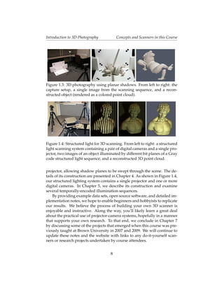
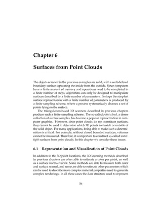
![Introduction to 3D Photography 3D Scanning Technology
Figure 1.1: Contact-based shape measurement. (Left) A sketch of Soren-
son’s engraving pantograph patented in 1867. (Right) A modern coordi-
nate measuring machining (from Flickr user hyperbolation). In both de-
vices, deflection of a probe tip is used to estimate object shape, either for
transferring engravings or for recovering 3D models, respectively.
drawn from each camera’s center of projection through the 3D point. The
intersection of these two lines is then used to recover the depth of the point.
Trinocular [VF92] and multi-view stereo [HZ04] systems have been in-
troduced to improve the accuracy and reliability of conventional stereo-
scopic systems. However, all such passive triangulation methods require
correspondences to be found among the various viewpoints. Even for stereo
vision, the development of matching algorithms remains an open and chal-
lenging problem in the field [SCD∗ 06]. Today, real-time stereoscopic and
multi-view systems are emerging, however certain challenges continue to
limit their widespread adoption [MPL04]. Foremost, flat or periodic tex-
tures prevent robust matching. While machine learning methods and prior
knowledge are being advanced to solve such problems, multi-view 3D scan-
ning remains somewhat outside the domain of hobbyists primarily con-
cerned with accurate, reliable 3D measurement.
Many alternative passive methods have been proposed to sidestep the
correspondence problem, often times relying on more robust computer vi-
sion algorithms. Under controlled conditions, such as a known or constant
background, the external boundaries of foreground objects can be reliably
identified. As a result, numerous shape-from-silhouette algorithms have
emerged. Laurentini [Lau94] considers the case of a finite number of cam-
eras observing a scene. The visual hull is defined as the union of the gener-
3](https://image.slidesharecdn.com/byo3d-090819162830-phpapp01/85/Build-Your-Own-3D-Scanner-Course-Notes-10-320.jpg)
![Introduction to 3D Photography 3D Scanning Technology
alized viewing cones defined by each camera’s center of projection and the
detected silhouette boundaries. Recently, free-viewpoint video [CTMS03]
systems have applied this algorithm to allow dynamic adjustment of view-
point [MBR∗ 00, SH03]. Cipolla and Giblin [CG00] consider a differential
formulation of the problem, reconstructing depth by observing the visual
motion of occluding contours (such as silhouettes) as a camera is perturbed.
Optical imaging systems require a sufficiently large aperture so that
enough light is gathered during the available exposure time [Hec01]. Cor-
respondingly, the captured imagery will demonstrate a limited depth of
field; only objects close to the plane of focus will appear in sharp contrast,
with distant objects blurred together. This effect can be exploited to recover
depth, by increasing the aperture diameter to further reduce the depth of
field. Nayar and Nakagawa [NN94] estimate shape-from-focus, collecting
a focal stack by translating a single element (either the lens, sensor, or ob-
ject). A focus measure operator [WN98] is then used to identify the plane
of best focus, and its corresponding distance from the camera.
Other passive imaging systems further exploit the depth of field by
modifying the shape of the aperture. Such modifications are performed
so that the point spread function (PSF) becomes invertible and strongly
depth-dependent. Levin et al. [LFDF07] and Farid [Far97] use such coded
apertures to estimate intensity and depth from defocused images. Green-
gard et al. [GSP06] modify the aperture to produce a PSF whose rotation is
a function of scene depth. In a similar vein, shadow moir´ is produced by
e
placing a high-frequency grating between the scene and the camera. The
resulting interference patterns exhibit a series of depth-dependent fringes.
While the preceding discussion focused on optical modifications for 3D
reconstruction from 2D images, numerous model-based approaches have
also emerged. When shape is known a priori, then coarse image measure-
ments can be used to infer object translation, rotation, and deformation.
Such methods have been applied to human motion tracking [KM00, OSS∗ 00,
dAST∗ 08], vehicle recognition [Sul95, FWM98], and human-computer in-
teraction [RWLB01]. Additionally, user-assisted model construction has
been demonstrated using manual labeling of geometric primitives [Deb97].
1.1.2 Active Methods
Active optical scanners overcome the correspondence problem using con-
trolled illumination. In comparison to non-contact and passive methods,
active illumination is often more sensitive to surface material properties.
Strongly reflective or translucent objects often violate assumptions made
4](https://image.slidesharecdn.com/byo3d-090819162830-phpapp01/85/Build-Your-Own-3D-Scanner-Course-Notes-11-320.jpg)
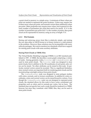
![Introduction to 3D Photography 3D Scanning Technology
Figure 1.2: Active methods for 3D scanning. (Left) Conceptual diagram
of a 3D slit scanner, consisting of a mechanically translated laser stripe.
(Right) A Cyberware scanner, applying laser striping for whole body scan-
ning (from Flickr user NIOSH).
by active optical scanners, requiring additional measures to acquire such
problematic subjects. For a detailed history of active methods, we refer the
reader to the survey article by Blais [Bla04]. In this section we discuss some
key milestones along the way to the scanners we consider in this course.
Many active systems attempt to solve the correspondence problem by
replacing one of the cameras, in a passive stereoscopic system, with a con-
trollable illumination source. During the 1970s, single-point laser scanning
emerged. In this scheme, a series of fixed and rotating mirrors are used to
raster scan a single laser spot across a surface. A digital camera records the
motion of this “flying spot”. The 2D projection of the spot defines, with
appropriate calibration knowledge, a line connecting the spot and the cam-
era’s center of projection. The depth is recovered by intersecting this line
with the line passing from the laser source to the spot, given by the known
deflection of the mirrors. As a result, such single-point scanners can be seen
as the optical equivalent of coordinate measuring machines.
As with CMMs, single-point scanning is a painstakingly slow process.
With the development of low-cost, high-quality CCD arrays in the 1980s,
slit scanners emerged as a powerful alternative. In this design, a laser pro-
jector creates a single planar sheet of light. This “slit” is then mechanically-
swept across the surface. As before, the known deflection of the laser
source defines a 3D plane. The depth is recovered by the intersection of
this plane with the set of lines passing through the 3D stripe on the surface
and the camera’s center of projection.
5](https://image.slidesharecdn.com/byo3d-090819162830-phpapp01/85/Build-Your-Own-3D-Scanner-Course-Notes-12-320.jpg)
![Introduction to 3D Photography 3D Scanning Technology
Effectively removing one dimension of the raster scan, slit scanners re-
main a popular solution for rapid shape acquisition. A variety of com-
mercial products use swept-plane laser scanning, including the Polhemus
FastSCAN [Pol], the NextEngine [Nex], the SLP 3D laser scanning probes
from Laser Design [Las], and the HandyScan line of products [Cre]. While
effective, slit scanners remain difficult to use if moving objects are present
in the scene. In addition, because of the necessary separation between the
light source and camera, certain occluded regions cannot be reconstructed.
This limitation, while shared by many 3D scanners, requires multiple scans
to be merged—further increasing the data acquisition time.
A digital “structured light” projector can be used to eliminate the me-
chanical motion required to translate the laser stripe across the surface.
Na¨vely, the projector could be used to display a single column (or row)
ı
of white pixels translating against a black background to replicate the per-
formance of a slit scanner. However, a simple swept-plane sequence does
not fully exploit the projector, which is typically capable of displaying ar-
bitrary 24-bit color images. Structured lighting sequences have been de-
veloped which allow the projector-camera correspondences to be assigned
in relatively few frames. In general, the identity of each plane can be en-
coded spatially (i.e., within a single frame) or temporally (i.e., across multi-
ple frames), or with a combination of both spatial and temporal encodings.
There are benefits and drawbacks to each strategy. For instance, purely
spatial encodings allow a single static pattern to be used for reconstruction,
enabling dynamic scenes to be captured. Alternatively, purely temporal en-
codings are more likely to benefit from redundancy, reducing reconstruc-
tion artifacts. We refer the reader to a comprehensive assessment of such
codes by Salvi et al. [SPB04].
Both slit scanners and structured lighting are ill-suited for scanning dy-
namic scenes. In addition, due to separation of the light source and cam-
era, certain occluded regions will not be recovered. In contrast, time-of-
flight rangefinders estimate the distance to a surface from a single center
of projection. These devices exploit the finite speed of light. A single pulse
of light is emitted. The elapsed time, between emitting and receiving a
pulse, is used to recover the object distance (since the speed of light is
known). Several economical time-of-flight depth cameras are now com-
mercially available, including Canesta’s CANESTAVISION [HARN06] and
3DV’s Z-Cam [IY01]. However, the depth resolution and accuracy of such
systems (for static scenes) remain below that of slit scanners and structured
lighting.
Active imaging is a broad field; a wide variety of additional schemes
6](https://image.slidesharecdn.com/byo3d-090819162830-phpapp01/85/Build-Your-Own-3D-Scanner-Course-Notes-13-320.jpg)
![Introduction to 3D Photography Concepts and Scanners in this Course
have been proposed, typically trading system complexity for shape ac-
curacy. As with model-based approaches in passive imaging, several ac-
tive systems achieve robust reconstruction by making certain simplifying
assumptions about the topological and optical properties of the surface.
Woodham [Woo89] introduces photometric stereo, allowing smooth sur-
faces to be recovered by observing their shading under at least three (spa-
tially disparate) point light sources. Hern´ ndez et al. [HVB∗ 07] further
a
demonstrate a real-time photometric stereo system using three colored light
sources. Similarly, the complex digital projector required for structured
lighting can be replaced by one or more printed gratings placed next to the
projector and camera. Like shadow moir´ , such projection moir´ systems
e e
create depth-dependent fringes. However, certain ambiguities remain in
the reconstruction unless the surface is assumed to be smooth.
Active and passive 3D scanning methods continue to evolve, with re-
cent progress reported annually at various computer graphics and vision
conferences, including 3-D Digital Imaging and Modeling (3DIM), SIG-
GRAPH, Eurographics, CVPR, ECCV, and ICCV. Similar advances are also
published in the applied optics communities, typically through various
SPIE and OSA journals. We will survey several promising recent works
in Chapter 7.
1.2 Concepts and Scanners in this Course
This course is grounded in the unifying concept of triangulation. At their
core, stereoscopic imaging, slit scanning, and structured lighting all at-
tempt to recover the shape of 3D objects in the same manner. First, the
correspondence problem is solved, either by a passive matching algorithm
or by an active “space-labeling” approach (e.g., projecting known lines,
planes, or other patterns). After establishing correspondences across two
or more views (e.g., between a pair of cameras or a single projector-camera
pair), triangulation recovers the scene depth. In stereoscopic and multi-
view systems, a point is reconstructed by intersecting two or more corre-
sponding lines. In slit scanning and structured lighting systems, a point is
recovered by intersecting corresponding lines and planes.
To elucidate the principles of such triangulation-based scanners, this
course describes how to construct classic slit scanners, as well as a struc-
tured lighting system. As shown in Figure 1.3, our slit scanner is inspired
by the work of Bouguet and Perona [BP]. In this design, a wooden stick and
halogen lamp replicate the function of a manually-translated laser stripe
7](https://image.slidesharecdn.com/byo3d-090819162830-phpapp01/85/Build-Your-Own-3D-Scanner-Course-Notes-14-320.jpg)
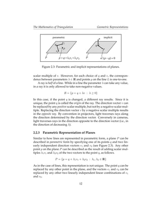
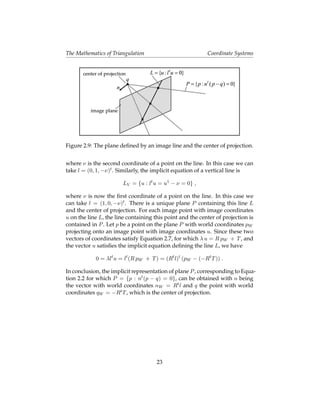
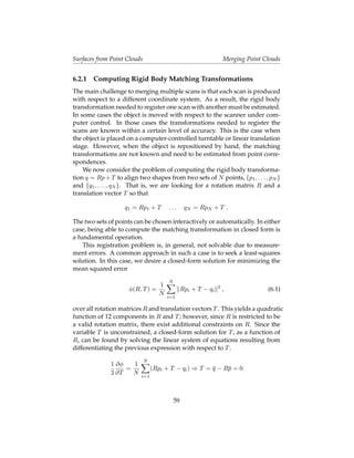
![The Mathematics of Triangulation Geometric Representations
center of projection
image plane
image
point
light direction
for a projector
3D point
light direction
for a camera
Figure 2.1: Perspective projection under the pinhole model.
from a projector (or towards a camera) along the line connecting the 3D
scene point with its 2D perspective projection onto the image plane.
2.2 Geometric Representations
Since light moves along straight lines (in a homogeneous medium such as
air), we derive 3D reconstruction equations from geometric constructions
involving the intersection of lines and planes, or the approximate intersec-
tion of pairs of lines (two lines in 3D may not intersect). Our derivations
only draw upon elementary algebra and analytic geometry in 3D (e.g., we
operate on points, vectors, lines, rays, and planes). We use lower case let-
ters to denote points p and vectors v. All the vectors will be taken as column
vectors with real-valued coordinates v ∈ IR3 , which we can also regard as
matrices with three rows and one column v ∈ IR3×1 . The length of a vector
v is a scalar v ∈ IR. We use matrix multiplication notation for the inner
t
product v1 v2 ∈ IR of two vectors v1 and v2 , which is also a scalar. Here
v1t ∈ IR1×3 is a row vector, or a 1 × 3 matrix, resulting from transposing
the column vector v1 . The value of the inner product of the two vectors v1
and v2 is equal to v1 v2 cos(α), where α is the angle formed by the two
vectors (0 ≤ α ≤ 180◦ ). The 3 × N matrix resulting from concatenating N
vectors v1 , . . . , vN as columns is denoted [v1 | · · · |vN ] ∈ IR3×N . The vector
product v1 × v2 ∈ IR3 of the two vectors v1 and v2 is a vector perpendicu-
lar to both v1 and v2 , of length v1 × v2 = v1 v2 sin(α), and direction
determined by the right hand rule (i.e., such that the determinant of the
10](https://image.slidesharecdn.com/byo3d-090819162830-phpapp01/85/Build-Your-Own-3D-Scanner-Course-Notes-17-320.jpg)
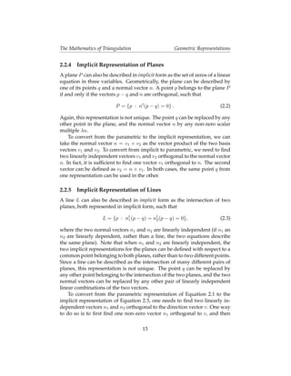
![The Mathematics of Triangulation Geometric Representations
p = q + λv p = q + λv
v
v
q
line ray
q
Figure 2.2: Parametric representation of lines and rays.
matrix [v1 |v2 |v1 × v2 ] is non-negative). In particular, two vectors v1 and v2
are linearly dependent ( i.e., one is a scalar multiple of the other), if and
only if the vector product v1 × v2 is equal to zero.
2.2.1 Points and Vectors
Since vectors form a vector space, they can be multiplied by scalars and
added to each other. Points, on the other hand, do not form a vector space.
But vectors and points are related: a point plus a vector p + v is another
point, and the difference between two points q − p is a vector. If p is a point,
λ is a scalar, and v is a vector, then q = p + λv is another point. In this
expression, λv is a vector of length |λ| v . Multiplying a point by a scalar
λp is not defined, but an affine combination of N points λ1 p1 + · · · + λN pN ,
with λ1 + · · · + λN = 1, is well defined:
λ1 p1 + · · · + λN pN = p1 + λ2 (p2 − p1 ) + · · · + λN (pN − p1 ) .
2.2.2 Parametric Representation of Lines and Rays
A line L can be described by specifying one of its points q and a direction
vector v (see Figure 2.2). Any other point p on the line L can be described
as the result of adding a scalar multiple λv, of the direction vector v, to the
point q (λ can be positive, negative, or zero):
L = {p = q + λv : λ ∈ IR} . (2.1)
This is the parametric representation of a line, where the scalar λ is the pa-
rameter. Note that this representation is not unique, since q can be replaced
by any other point on the line L, and v can be replaced by any non-zero
11](https://image.slidesharecdn.com/byo3d-090819162830-phpapp01/85/Build-Your-Own-3D-Scanner-Course-Notes-18-320.jpg)
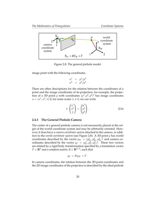
![The Mathematics of Triangulation Coordinate Systems
camera coordinate system
q=0 u1 p1
v2 v3 u = u2 p = p2
v1
1 3
p
f =1 world coordinate system
Figure 2.7: The ideal pinhole camera.
2.4.1 Image Coordinates and the Pinhole Camera
Consider a pinhole model with center of projection o and image plane P =
{p = q + u1 v1 + u2 v2 : u1 , u2 ∈ IR}. Any 3D point p, not necessarily on
the image plane, has coordinates (p1 , p2 , p3 )t relative to the origin of the
world coordinate system. On the image plane, the point q and vectors v1
and v2 define a local coordinate system. The image coordinates of a point
p = q + u1 v1 + u2 v2 are the parameters u1 and u2 , which can be written as
a 3D vector u = (u1 , u2 , 1). Using this notation point p is expressed as
1 1
p u
p2 = [v1 |v2 |q] u2 .
p3 1
2.4.2 The Ideal Pinhole Camera
In the ideal pinhole camera shown in Figure 2.7, the center of projection o is
at the origin of the world coordinate system, with coordinates (0, 0, 0)t , and
the point q and the vectors v1 and v2 are defined as
1 0 0
[v1 |v2 |q] = 0 1 0 .
0 0 1
Note that not every 3D point has a projection on the image plane. Points
without a projection are contained in a plane parallel to the image passing
through the center of projection. An arbitrary 3D point p with coordinates
(p1 , p2 , p3 )t belongs to this plane if p3 = 0, otherwise it projects onto an
19](https://image.slidesharecdn.com/byo3d-090819162830-phpapp01/85/Build-Your-Own-3D-Scanner-Course-Notes-26-320.jpg)
![Chapter 3
Camera and Projector Calibration
Triangulation is a deceptively simple concept, simply involving the pair-
wise intersection of 3D lines and planes. Practically, however, one must
carefully calibrate the various cameras and projectors so the equations of
these geometric primitives can be recovered from image measurements. In
this chapter we lead the reader through the construction and calibration of
a basic projector-camera system. Through this example, we examine how
freely-available calibration packages, emerging from the computer vision
community, can be leveraged in your own projects. While touching on the
basic concepts of the underlying algorithms, our primarily goal is to help
beginners overcome the “calibration hurdle”.
In Section 3.1 we describe how to select, control, and calibrate a dig-
ital camera suitable for 3D scanning. The general pinhole camera model
presented in Chapter 2 is extended to address lens distortion. A simple cal-
ibration procedure using printed checkerboard patterns is presented, fol-
lowing the established method of Zhang [Zha00]. Typical calibration re-
sults, obtained for the cameras used in Chapters 4 and 5, are provided as a
reference.
While well-documented, freely-available camera calibration tools have
emerged in recent years, community tools for projector calibration have re-
ceived significantly less attention. In Section 3.2, we describe custom pro-
jector calibration software developed for this course. A simple procedure
is used, wherein a calibrated camera observes a planar object with both
printed and projected checkerboards on its surface. Considering the projec-
tor as an inverse camera, we describe how to estimate the various parame-
ters of the projection model from such imagery. We conclude by reviewing
calibration results for the structured light projector used in Chapter 5.
24](https://image.slidesharecdn.com/byo3d-090819162830-phpapp01/85/Build-Your-Own-3D-Scanner-Course-Notes-31-320.jpg)
![Camera and Projector Calibration Camera Calibration
3.1 Camera Calibration
In this section we describe both the theory and practice of camera calibra-
tion. We begin by briefly considering what cameras are best suiting for
building your own 3D scanner. We then present the widely-used calibra-
tion method originally proposed by Zhang [Zha00]. Finally, we provide
step-by-step directions on how to use a freely-available M ATLAB-based im-
plementation of Zhang’s method.
3.1.1 Camera Selection and Interfaces
Selection of the “best” camera depends on your budget, project goals, and
preferred development environment. For instance, the two scanners de-
scribed in this course place different restrictions on the imaging system.
The swept-plane scanner in Chapter 4 requires a video camera, although
a simple camcorder or webcam would be sufficient. In contrast, the struc-
tured lighting system in Chapter 5 can be implemented using a still cam-
era. However, the camera must allow computer control of the shutter so
image capture can be synchronized with image projection. In both cases,
the range of cameras are further restricted to those that are supported by
your development environment.
At the time of writing, the accompanying software for this course was
primarily written in M ATLAB. If readers wish to collect their own data sets
using our software, we recommend obtaining a camera supported by the
Image Acquisition Toolbox for M ATLAB [Mat]. Note that this toolbox sup-
ports products from a variety of vendors, as well as any DCAM-compatible
FireWire camera or webcam with a Windows Driver Model (WDM) or
Video for Windows (VFW) driver. For FireWire cameras the toolbox uses
the CMU DCAM driver [CMU]. Alternatively, if you select a WDM or VFW
camera, Microsoft DirectX 9.0 (or higher) must be installed.
If you do not have access to any camera meeting these constraints, we
recommend either purchasing an inexpensive FireWire camera or a high-
quality USB webcam. While most webcams provide compressed imagery,
FireWire cameras typically allow access to raw images free of compression
artifacts. For those on a tight budget, we recommend the Unibrain Fire-i
(available for around $100 USD). Although more expensive, we also recom-
mend cameras from Point Grey Research. The camera interface provided
by this vendor is particularly useful if you plan on developing more ad-
vanced scanners than those presented here. As a point of reference, our
scanners were built using a pair of Point Grey GRAS-20S4M/C Grasshop-
25](https://image.slidesharecdn.com/byo3d-090819162830-phpapp01/85/Build-Your-Own-3D-Scanner-Course-Notes-32-320.jpg)
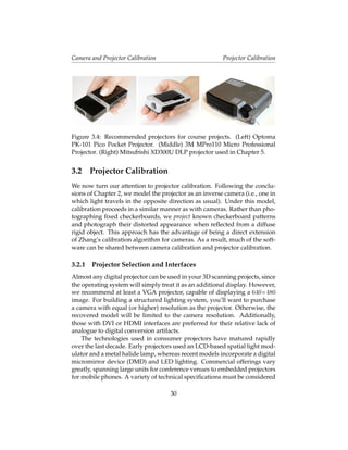
![Camera and Projector Calibration Camera Calibration
Figure 3.1: Recommended cameras for course projects. (Left) Unibrain Fire-
i IEEE-1394a digital camera, capable of 640×480 YUV 4:2:2 capture at 15
fps. (Middle) Logitech QuickCam Orbit AF USB 2.0 webcam, capable of
1600×1200 image capture at 30 fps. (Right) Point Grey Grasshopper IEEE-
1394b digital camera; frame rate and resolution vary by model.
per video cameras. Each camera can capture a 1600×1200 24-bit RGB image
at up to 30 Hz [Poia].
Outside of M ATLAB, a wide variety of camera interfaces are available.
However, relatively few come with camera calibration software, and even
fewer with support for projector calibration. One exception, however, is
the OpenCV (Open Source Computer Vision) library [Opea]. OpenCV is
written in C, with wrappers for C# and Python, and consists of optimized
implementations of many core computer vision algorithms. Video capture
and display functions support a wide variety of cameras under multiple
operating systems, including Windows, Mac OS, and Linux. Note, how-
ever, that projector calibration is not currently supported in OpenCV.
3.1.2 Calibration Methods and Software
Camera Calibration Methods
Camera calibration requires estimating the parameters of the general pin-
hole model presented in Section 2.4.3. This includes the intrinsic parame-
ters, being focal length, principal point, and the scale factors, as well as the
extrinsic parameters, defined by the rotation matrix and translation vector
mapping between the world and camera coordinate systems. In total, 11
parameters (5 intrinsic and 6 extrinsic) must be estimated from a calibra-
tion sequence. In practice, a lens distortion model must be estimated as
well. We recommend the reader review [HZ04, MSKS05] for an in-depth
description of camera models and calibration methods.
26](https://image.slidesharecdn.com/byo3d-090819162830-phpapp01/85/Build-Your-Own-3D-Scanner-Course-Notes-33-320.jpg)
![Camera and Projector Calibration Camera Calibration
At a basic level, camera calibration required recording a sequence of
images of a calibration object, composed of a unique set of distinguishable
features with known 3D displacements. Thus, each image of the calibration
object provides a set of 2D-to-3D correspondences, mapping image coordi-
nates to scene points. Na¨vely, one would simply need to optimize over the
ı
set of 11 camera model parameters so that the set of 2D-to-3D correspon-
dences are correctly predicted (i.e., the projection of each known 3D model
feature is close to its measured image coordinates).
Many methods have been proposed over the years to solve for the cam-
era parameters given such correspondences. In particular, the factorized
approach originally proposed Zhang [Zha00] is widely-adopted in most
community-developed tools. In this method, a planar checkerboard pat-
tern is observed in two or more orientations (see Figure 3.2). From this
sequence, the intrinsic parameters can be separately solved. Afterwards,
a single view of a checkerboard can be used to solve for the extrinsic pa-
rameters. Given the relative ease of printing 2D patterns, this method is
commonly used in computer graphics and vision publications.
Recommended Software
A comprehensive list of calibration software is maintained by Bouguet on
the toolbox website at http://www.vision.caltech.edu/bouguetj/
calib_doc/htmls/links.html. We recommend course attendees use
the M ATLAB toolbox. Otherwise, OpenCV replicates many of its function-
alities, while supporting multiple platforms. Although calibrating a small
number of cameras using these tools is straightforward, calibrating a large
network of cameras is a relatively recent and challenging problem in the
field. If your projects lead you in this direction, we suggest the Multi-
Camera Self-Calibration toolbox [SMP05]. This software takes a unique ap-
proach to calibration; rather than using multiple views of a planar calibra-
tion object, a standard laser point is simply translated through the working
volume. Correspondences between the cameras are automatically deter-
mined from the tracked projection of the laser pointer in each image. We
encourage attendees to email us with their own preferred tools. We will
maintain an up-to-date list on the course website. For the remainder of the
course notes, we will use the M ATLAB toolbox for camera calibration.
27](https://image.slidesharecdn.com/byo3d-090819162830-phpapp01/85/Build-Your-Own-3D-Scanner-Course-Notes-34-320.jpg)
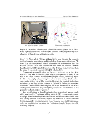
![Camera and Projector Calibration Camera Calibration
Figure 3.2: Camera calibration sequence containing multiple views of a
checkerboard at various positions and orientations throughout the scene.
3.1.3 Calibration Procedure
In this section we describe, step-by-step, how to calibrate your camera us-
ing the Camera Calibration Toolbox for M ATLAB. We also recommend re-
viewing the detailed documentation and examples provided on the toolbox
website [Bou]. Specifically, new users should work through the first cali-
bration example and familiarize themselves with the description of model
parameters (which differ slightly from the notation used in these notes).
Begin by installing the toolbox, available for download at http://
www.vision.caltech.edu/bouguetj/calib_doc/. Next, construct
a checkerboard target. Note that the toolbox comes with a sample checker-
board image; print this image and affix it to a rigid object, such as piece
of cardboard or textbook cover. Record a series of 10–20 images of the
checkerboard, varying its position and pose between exposures. Try to col-
lect images where the checkerboard is visible throughout the image.
Using the toolbox is relatively straightforward. Begin by adding the
toolbox to your M ATLAB path by selecting “File → Set Path...”. Next,
change the current working directory to one containing your calibration
images (or one of our test sequences). Type calib at the M ATLAB prompt
to start. Since we’re only using a few images, select “Standard (all the im-
ages are stored in memory)” when prompted. To load the images, select
“Image names” and press return, then “j”. Now select “Extract grid cor-
ners”, pass through the prompts without entering any options, and then
follow the on-screen directions. (Note that the default checkerboard has
30mm×30mm squares). Always skip any prompts that appear, unless you
are more familiar with the toolbox options. Once you’ve finished selecting
28](https://image.slidesharecdn.com/byo3d-090819162830-phpapp01/85/Build-Your-Own-3D-Scanner-Course-Notes-35-320.jpg)
![Camera and Projector Calibration Projector Calibration
when choosing the “best” projector for your 3D scanning projects. Varia-
tions in throw distance (i.e., where focused images can be formed), projec-
tor artifacts (i.e., pixelization and distortion), and cost are key factors.
Digital projectors have a tiered pricing model, with brighter projectors
costing significantly more than dimmer ones. At the time of writing, a
1024×768 projector can be purchased for around $400–$600 USD. Most
models in this price bracket have a 1000:1 contrast ratio with an output
around 2000 ANSI lumens. Note that this is about as bright as a typical
100 W incandescent light bulb. Practically, such projectors are sufficient for
projecting a 100 inch (diagonal) image in a well-lit room.
For those on a tighter budget, we recommend purchasing a hand-held
projector. Also known as ”pocket” projectors, these miniaturized devices
typically use DMD or LCoS technology together with LED lighting. Cur-
rent offerings include the 3M MPro, Aiptek V10, Aaxatech P1, and Optoma
PK101, with prices around $300 USD. While projectors in this class typically
output only 10 lumens, this is sufficient to project up to a 50 inch (diago-
nal) image (in a darkened room). However, we recommend a higher-lumen
projector if you plan on scanning large objects in well-lit environments.
While your system will consider the projector as a second display, your
development environment may or may not easily support fullscreen dis-
play. For instance, M ATLAB does not natively support fullscreen display
(i.e., without window borders or menus). One solution is to use Java dis-
play functions, with which the M ATLAB GUI is built. Code for this ap-
proach is available at http://www.mathworks.com/matlabcentral/
fileexchange/11112. Unfortunately, we found that this approach only
works for the primary display. As an alternative, we recommend using
the Psychophysics Toolbox [Psy]. While developed for a different applica-
tion, this toolbox contains OpenGL wrappers allowing simple and direct
fullscreen control of the system displays from M ATLAB. For details, please
see our structured light source code. Finally, for users working outside of
M ATLAB, we recommend controlling projectors through OpenGL.
3.2.2 Calibration Methods and Software
Projector calibration has received increasing attention, in part driven by
the emergence of lower-cost digital projectors. As mentioned at several
points, a projector is simply the “inverse” of a camera, wherein points on an
image plane are mapped to outgoing light rays passing through the center
of projection. As in Section 3.1.2, a lens distortion model can augment the
basic general pinhole model presented in Chapter 2.
31](https://image.slidesharecdn.com/byo3d-090819162830-phpapp01/85/Build-Your-Own-3D-Scanner-Course-Notes-38-320.jpg)
![Camera and Projector Calibration Projector Calibration
Figure 3.5: Projector calibration sequence containing multiple views of a
checkerboard projected on a white plane marked with four printed fidu-
cials in the corners. As for camera calibration, the plane must be moved to
various positions and orientations throughout the scene.
Numerous methods have been proposed for estimating the parameters
of this inverse camera model. However, community-developed tools are
slow to emerge—most researchers keeping their tools in-house. It is our
opinion that both OpenCV and the M ATLAB calibration toolbox can be eas-
ily modified to allow projector calibration. We document our modifica-
tions to the latter in the following section. As noted in the OpenCV text-
book [BK08], it is expected that similar modifications to OpenCV (possibly
arising from this course’s attendees) will be made available soon.
3.2.3 Calibration Procedure
In this section we describe, step-by-step, how to calibrate your projector us-
ing our software, which is built on top of the Camera Calibration Toolbox
for M ATLAB. Begin by calibrating your camera(s) using the procedure out-
lined in the previous section. Next, install the toolbox extensions available
on the course website at http://mesh.brown.edu/dlanman/scan3d.
Construct a calibration object similar to those in Figures 3.5 and 3.6. This
object should be a diffuse white planar object, such as foamcore or a painted
piece of particle board. Printed fiducials, possibly cut from a section of your
camera calibration pattern, should be affixed to the surface. One option is
to simply paste a section of the checkerboard pattern in one corner. In our
implementation we place four checkerboard corners at the edges of the cal-
ibration object. The distances and angles between these points should be
recorded.
32](https://image.slidesharecdn.com/byo3d-090819162830-phpapp01/85/Build-Your-Own-3D-Scanner-Course-Notes-39-320.jpg)
![Camera and Projector Calibration Projector Calibration
(a) projector calibration (b) projector lens distortion
Figure 3.6: Estimating the intrinsic parameters of the projector using a cali-
brated camera. (a) Calibration image collected using a white plane marked
with four fiducials in the corners (denoted as red circles). (b) The resulting
fourth-order lens distortion model for the projector.
A known checkerboard must be projected onto the calibration object.
We have provided run capture to generate the checkerboard pattern,
as well as collect the calibration sequence. As previously mentioned, this
script controls the projector using the Psychophysics Toolbox [Psy]. A se-
ries of 10–20 images should be recorded by projecting the checkerboard
onto the calibration object. Suitable calibration images are shown in Fig-
ure 3.5. Note that the printed fiducials must be visible in each image and
that the projected checkerboard should not obscure them. There are a vari-
ety of methods to prevent projected and printed checkerboards from inter-
fering; one solution is to use color separation (e.g., printed and projected
checkerboards in red and blue, respectively), however this requires the
camera be color calibrated. We encourage you to try a variety of options
and send us your results for documentation on the course website.
Your camera calibration images should be stored in the cam subdirec-
tory of the provided projector calibration package. The calib data.mat
file, produced by running camera calibration, should be stored in this di-
rectory as well. The projector calibration images should be stored in the
proj subdirectory. Afterwards, run the camera calibration toolbox by typing
calib at the M ATLAB prompt (in this directory). Since we’re only using a
few images, select “Standard (all the images are stored in memory)” when
prompted. To load the images, select “Image names” and press return,
33](https://image.slidesharecdn.com/byo3d-090819162830-phpapp01/85/Build-Your-Own-3D-Scanner-Course-Notes-40-320.jpg)
![Chapter 4
3D Scanning with Swept-Planes
In this chapter we describe how to build an inexpensive, yet accurate, 3D
scanner using household items and a digital camera. Specifically, we’ll de-
scribe the implementation of the “desktop scanner” originally proposed by
Bouguet and Perona [BP]. As shown in Figure 4.1, our instantiation of this
system is composed of five primary items: a digital camera, a point-like
light source, a stick, two planar surfaces, and a calibration checkerboard.
By waving the stick in front of the light source, the user can cast planar
shadows into the scene. As we’ll demonstrate, the depth at each pixel can
then be recovered using simple geometric reasoning.
In the course of building your own “desktop scanner” you will need to
develop a good understanding of camera calibration, Euclidean coordinate
transformations, manipulation of implicit and parametric parameteriza-
tions of lines and planes, and efficient numerical methods for solving least-
squares problems—topics that were previously presented in Chapter 2. We
encourage the reader to also review the original project website [BP] and
obtain a copy of the IJCV publication [BP99], both of which will be referred
to several times throughout this chapter. Also note that the software accom-
panying this chapter was developed in M ATLAB at the time of writing. We
encourage the reader to download that version, as well as updates, from
the course website at http://mesh.brown.edu/dlanman/scan3d.
4.1 Data Capture
As shown in Figure 4.1, the scanning apparatus is simple to construct and
contains relatively few components. A pair of blank white foamcore boards
are used as planar calibration objects. These boards can be purchased at an
35](https://image.slidesharecdn.com/byo3d-090819162830-phpapp01/85/Build-Your-Own-3D-Scanner-Course-Notes-42-320.jpg)
![3D Scanning with Swept-Planes Data Capture
(a) swept-plane scanning apparatus (b) frame from acquired video sequence
Figure 4.1: 3D photography using planar shadows. (a) The scanning setup,
composed of five primary items: a digital camera, a point-like light source,
a stick, two planar surfaces, and a calibration checkerboard (not shown).
Note that the light source and camera must be separated so that cast
shadow planes and camera rays do not meet at small incidence angles. (b)
The stick is slowly waved in front of the point light to cast a planar shadow
that translates from left to right in the scene. The position and orientation
of the shadow plane, in the world coordinate system, are estimated by ob-
serving its position on the planar surfaces. After calibrating the camera,
a 3D model can be recovered by triangulation of each optical ray by the
shadow plane that first entered the corresponding scene point.
art supply store. Any rigid light-colored planar object could be substituted,
including particle board, acrylic sheets, or even lightweight poster board.
At least four fiducials, such as the printed checkerboard corners shown in
the figure, should be affixed to known locations on each board. The dis-
tance and angle between each fiducial should be measured and recorded
for later use in the calibration phase. These measurements will allow the
position and orientation of each board to be estimated in the world coor-
dinate system. Finally, the boards should be oriented approximately at a
right angle to one another.
Next, a planar light source must be constructed. In this chapter we will
follow the method of Bouguet and Perona [BP], in which a point source
and a stick are used to cast planar shadows. Wooden dowels of varying
diameter can be obtained at a hardware store, and the point light source
can be fashioned from any halogen desk lamp after removing the reflector.
Alternatively, a laser stripe scanner could be implemented by replacing the
36](https://image.slidesharecdn.com/byo3d-090819162830-phpapp01/85/Build-Your-Own-3D-Scanner-Course-Notes-43-320.jpg)
![3D Scanning with Swept-Planes Data Capture
point light source and stick with a modified laser pointer. In this case, a
cylindrical lens must be affixed to the exit aperture of the laser pointer,
creating a low-cost laser stripe projector. Both components can be obtained
from Edmund Optics [Edm]. For example, a section of a lenticular array or
cylindrical Fresnel lens sheet could be used. However, in the remainder of
this chapter we will focus on the shadow-casting method.
Any video camera or webcam can be used for image acquisition. The
light source and camera should be separated, so that the angle between
camera rays and cast shadow planes is close to perpendicular (otherwise
triangulation will result in large errors). Data acquisition is simple. First, an
object is placed on the horizontal calibration board, and the stick is slowly
translated in front of the light source (see Figure 4.1). The stick should be
waved such that a thin shadow slowly moves across the screen in one di-
rection. Each point on the object should be shadowed at some point during
data acquisition. Note that the camera frame rate will determine how fast
the stick can be waved. If it is moved too fast, then some pixels will not be
shadowed in any frame—leading to reconstruction artifacts.
We have provided several test sequences with our setup, which are
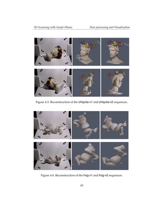
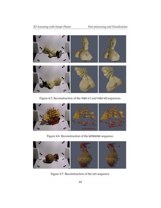
available on the course website [LT]. As shown in Figures 4.3–4.7, there are
a variety of objects available, ranging from those with smooth surfaces to
those with multiple self-occlusions. As we’ll describe in the following sec-
tions, reconstruction requires accurate estimates of the shadow boundaries.
As a result, you will find that light-colored objects (e.g., the chiquita, frog,
and man sequences) will be easiest to reconstruct. Since you’ll need to es-
timate the intrinsic and extrinsic calibration of the camera, we’ve also pro-
vided the calib sequence composed of ten images of a checkerboard with
various poses. For each sequence we have provided both a high-resolution
1024×768 sequence, as well as a low-resolution 512×384 sequence for de-
velopment.
When building your own scanning apparatus, briefly note some prac-
tical issues associated with this approach. First, it is important that every
pixel be shadowed at some point in the sequence. As a result, you must
wave the stick slow enough to ensure that this condition holds. In addition,
the reconstruction method requires reliable estimates of the plane defined
by the light source and the edge of the stick. Ambient illumination must be
reduced so that a single planar shadow is cast by each edge of the stick. In
addition, the light source must be sufficiently bright to allow the camera to
operate with minimal gain, otherwise sensor noise will corrupt the final re-
construction. Finally, note that these systems typically use a single halogen
desk lamp with the reflector removed. This ensures that the light source is
37](https://image.slidesharecdn.com/byo3d-090819162830-phpapp01/85/Build-Your-Own-3D-Scanner-Course-Notes-44-320.jpg)
![3D Scanning with Swept-Planes Video Processing
(a) spatial shadow edge localization (b) temporal shadow edge localization
Figure 4.2: Spatial and temporal shadow edge localization. (a) The shadow
edges are determined by fitting a line to the set of zero crossings, along
each row in the planar regions, of the difference image ∆I(x, y, t). (b) The
shadow times (quantized to 32 values here) are determined by finding the
zero-crossings of the difference image ∆I(x, y, t) for each pixel (x, y) as a
function of time t. Early to late shadow times are shaded from blue to red.
sufficiently point-like to produce abrupt shadow boundaries.
4.2 Video Processing
Two fundamental quantities must be estimated from a recorded swept-
plane video sequence: (1) the time that the shadow enters (and/or leaves)
each pixel and (2) the spatial position of each leading (and/or trailing)
shadow edge as a function of time. This section outlines the basic pro-
cedures for performing these tasks. Additional technical details are pre-
sented in Section 2.4 in [BP99] and Section 6.2.4 in [Bou99]. Our reference
implementation is provided in the videoProcessing m-file. Note that,
for large stick diameters, the shadow will be thick enough that two dis-
tinct edges can be resolved in the captured imagery. By tracking both the
leading and trailing shadow edges, two independent 3D reconstructions
are obtained—allowing robust outlier rejection and improved model qual-
ity. However, in a basic implementation, only one shadow edge must be
processed using the following methods. In this section we will describe
calibration of the leading edge, with a similar approach applying for the
trailing edge.
38](https://image.slidesharecdn.com/byo3d-090819162830-phpapp01/85/Build-Your-Own-3D-Scanner-Course-Notes-45-320.jpg)
![3D Scanning with Swept-Planes Video Processing
4.2.1 Spatial Shadow Edge Localization
To reconstruct a 3D model, we must know the equation of each shadow
plane in the world coordinate system. As shown in Figure 4.2, the cast
shadow will create four distinct lines in the camera image, consisting of a
pair of lines on both the horizontal and vertical calibration boards. These
lines represent the intersection of the 3D shadow planes (both the leading
and trailing edges) with the calibration boards. Using the notation of Figure
2 in [BP99], we need to estimate the 2D shadow lines λh (t) and λv (t) pro-
jected on the horizontal and vertical planar regions, respectively. In order to
perform this and subsequent processing, a spatio-temporal approach can be
used. As described in by Zhang et al. [ZCS03], this approach tends to pro-
duce better reconstruction results than traditional edge detection schemes
(e.g., the Canny edge detector [MSKS05]), since it is capable of preserving
sharp surface discontinuities.
Begin by converting the video to grayscale (if a color camera was used),
and evaluate the maximum and minimum brightness observed at each
camera pixel xc = (x, y) over the stick-waving sequence.
¯
Imax (x, y) max I(x, y, t)
t
Imin (x, y) min I(x, y, t)
t
To detect the shadow boundaries, choose a per-pixel detection threshold
which is the midpoint of the dynamic range observed in each pixel. With
this threshold, the shadow edge can be localized by the zero crossings of
the difference image
∆I(x, y, t) I(x, y, t) − Ishadow (x, y),
where the shadow threshold image is defined to be
Imax (x, y) + Imin (x, y)
Ishadow (x, y) .
2
In practice, you’ll need to select an occlusion-free image patch for each pla-
nar region. Afterwards, a set of sub-pixel shadow edge samples (for each
row of the patch) are obtained by interpolating the position of the zero-
crossings of ∆I(x, y, t). To produce a final estimate of the shadow edges
λh (t) and λv (t), the best-fit line (in the least-squares sense) must be fit to
the set of shadow edge samples. The desired output of this step is illus-
trated in Figure 4.2(a), where the best-fit lines are overlaid on the original
39](https://image.slidesharecdn.com/byo3d-090819162830-phpapp01/85/Build-Your-Own-3D-Scanner-Course-Notes-46-320.jpg)
![3D Scanning with Swept-Planes Calibration
image. Keep in mind that you should convert the provided color images to
grayscale; if you’re using M ATLAB, the function rgb2gray can be used for
this task.
4.2.2 Temporal Shadow Edge Localization
After calibrating the camera, the previous step will provide all the informa-
tion necessary to recover the position and orientation of each shadow plane
as a function of time in the world coordinate system. As we’ll describe in
Section 4.4, in order to reconstruct the object you’ll also need to know when
each pixel entered the shadowed region. This task can be accomplished in a
similar manner as spatial localization. Instead of estimating zero-crossing
along each row for a fixed frame, the per-pixel shadow time is assigned
using the zero crossings of the difference image ∆I(x, y, t) for each pixel
(x, y) as a function of time t. The desired output of this step is illustrated
in Figure 4.2(b), where the shadow crossing times are quantized to 32 val-
ues (with blue indicating earlier times and red indicated later ones). Note
that you may want to include some additional heuristics to reduce false de-
tections. For instance, dark regions cannot be reliably assigned a shadow
time. As a result, you can eliminate pixels with insufficient contrast (e.g.,
dark blue regions in the figure).
4.3 Calibration
As described in Chapters 2 and 3, intrinsic and extrinsic calibration of the
camera is necessary to transfer image measurements into the world coor-
dinate system. For the swept-plane scanner, we recommend using either
the Camera Calibration Toolbox for M ATLAB [Bou] or the calibration func-
tions within OpenCV [Opea]. As previously described, these packages are
commonly used within the computer vision community and, at their core,
implement the widely adopted calibration method originally proposed by
Zhang [Zha99]. In this scheme, the intrinsic and extrinsic parameters are
estimated by viewing several images of a planar checkerboard with var-
ious poses. In this section we will briefly review the steps necessary to
calibrate the camera using the M ATLAB toolbox. We recommend reviewing
the documentation on the toolbox website [Bou] for additional examples;
specifically, the first calibration example and the description of calibration
parameters are particularly useful to review for new users.
40](https://image.slidesharecdn.com/byo3d-090819162830-phpapp01/85/Build-Your-Own-3D-Scanner-Course-Notes-47-320.jpg)
![3D Scanning with Swept-Planes Reconstruction
4.4 Reconstruction
At this point, the system is fully calibrated. Specifically, optical rays pass-
ing through the camera’s center of projection can be expressed in the same
world coordinate system as the set of temporally-indexed shadow planes.
Ray-plane triangulation can now be applied to estimate the per-pixel depth
(at least for those pixels where the shadow was observed). In terms of Fig-
ure 2 in [BP99], the camera calibration is used to obtain a parametrization
of the ray defined by a true object point P and the camera center Oc . Given
the shadow time for the associated pixel xc , one can lookup (and potentially
¯
interpolate) the position of the shadow plane at this time. The resulting ray-
plane intersection will provide an estimate of the 3D position of the surface
point. Repeating this procedure for every pixel will produce a 3D recon-
struction. For complementary and extended details on the reconstruction
process, please consult Sections 2.5 and 2.6 in [BP99] and Sections 6.2.5 and
6.2.6 in [Bou99].
4.5 Post-processing and Visualization
Once you have reconstructed a 3D point cloud, you’ll want to visualize
the result. Regardless of the environment you used to develop your solu-
tion, you can write a function to export the recovered points as a VRML file
containing a single indexed face set with an empty coordIndex array. Ad-
ditionally, a per-vertex color can be assigned by sampling the maximum-
luminance color, observed over the video sequence. In Chapter 6 we docu-
ment further post-processing that can be applied, including merging mul-
tiple scans and extracting watertight meshes. However, the simple colored
point clouds produced at this stage can be rendered using the Java-based
point splatting software provided on the course website.
To give you some expectation of reconstruction quality, Figures 4.3–4.7
show results obtained with our reference implementation. Note that there
are several choices you can make in your implementation; some of these
may allow you to obtain additional points on the surface or increase the
reconstruction accuracy. For example, using both the leading and trail-
ing shadow edges will allow outliers to be rejected (by eliminating points
whose estimated depth disagrees between the leading vs. trailing shadow
edges).
42](https://image.slidesharecdn.com/byo3d-090819162830-phpapp01/85/Build-Your-Own-3D-Scanner-Course-Notes-49-320.jpg)
![Chapter 5
Structured Lighting
In this chapter we describe how to build a structured light scanner using
one or more digital cameras and a single projector. While the “desktop
scanner” [BP] implemented in the previous chapter is inexpensive, it has
limited practical utility. The scanning process requires manual manipula-
tion of the stick, and the time required to sweep the shadow plane across
the scene limits the system to reconstructing static objects. Manual transla-
tion can be eliminated by using a digital projector to sequentially display
patterns (e.g., a single stipe translated over time). Furthermore, various
structured light illumination sequences, consisting of a series of projected
images, can be used to efficiently solve for the camera pixel to projector
column (or row) correspondences.
By implementing your own structured light scanner, you will directly
extending the algorithms and software developed for the swept-plane sys-
tems in the previous chapter. Reconstruction will again be accomplished
using ray-plane triangulation. The key difference is that correspondences
will now be established by decoding certain structured light sequences. At
the time of writing, the software accompanying this chapter was devel-
oped in M ATLAB. We encourage the reader to download that version, as
well as any updates, from the course website at http://mesh.brown.
edu/dlanman/scan3d.
5.1 Data Capture
5.1.1 Scanner Hardware
As shown in Figure 5.1, the scanning apparatus contains one or more digi-
tal cameras and a single digital projector. As with the swept-plane systems,
45](https://image.slidesharecdn.com/byo3d-090819162830-phpapp01/85/Build-Your-Own-3D-Scanner-Course-Notes-52-320.jpg)
![Structured Lighting Data Capture
Figure 5.1: Structured light for 3D scanning. From left to right: a structured
light scanning system containing a pair of digital cameras and a single pro-
jector, two images of an object illuminated by different bit planes of a Gray
code structured light sequence, and a reconstructed 3D point cloud.
the object will eventually be reconstructed by ray-plane triangulation, be-
tween each camera ray and a plane corresponding to the projector column
(and/or row) illuminating that point on the surface. As before, the cam-
eras and projector should be arranged to ensure that no camera ray and
projector plane meet at small incidence angles. A “diagonal” placement of
the cameras, as shown in the figure, ensures that both projector rows and
columns can be used for reconstruction.
As briefly described in Chapter 3, a wide variety of digital cameras
and projectors can be selected for your implementation. While low-cost
webcams will be sufficient, access to raw imagery will eliminate decod-
ing errors introduced by compression artifacts. You will want to select a
camera that is be supported by your preferred development environment.
For example, if you plan on using the M ATLAB Image Acquisition Toolbox,
then any DCAM-compatible FireWire camera or webcam with a Windows
Driver Model (WDM) or Video for Windows (VFW) driver will work [Mat].
If you plan on developing in OpenCV, a list compatible cameras is main-
tained on the wiki [Opeb]. Almost any digital projector can be used, since
the operating system will simply treat it as an additional display.
As a point of reference, our implementation contains a single Mitsubishi
XD300U DLP projector and a pair of Point Grey GRAS-20S4M/C Grasshop-
per video cameras. The projector is capable of displaying 1024×768 24-bit
RGB images at 50-85 Hz [Mit]. The cameras capture 1600×1200 24-bit RGB
images at up to 30 Hz [Poia]. Although lower-resolution modes can be
used if higher frame rates are required. The data capture was implemented
in M ATLAB. The cameras were controlled using custom wrappers for the
FlyCapture SDK [Poib], and fullscreen control of the projector was achiev-
46](https://image.slidesharecdn.com/byo3d-090819162830-phpapp01/85/Build-Your-Own-3D-Scanner-Course-Notes-53-320.jpg)
![Structured Lighting Data Capture
ing using the Psychophysics Toolbox [Psy] (see Chapter 3).
5.1.2 Structured Light Sequences
The primary benefit of introducing the projector is to eliminate the mechan-
ical motion required in swept-plane scanning systems (e.g., laser striping
or the “desktop scanner”). Assuming minimal lens distortion, the projector
can be used to display a single column (or row) of white pixels translating
against a black background; thus, 1024 (or 768) images would be required
to assign the correspondences, in our implementation, between camera pix-
els and projector columns (or rows). After establishing the correspondences
and calibrating the system, a 3D point cloud is reconstructed using familiar
ray-plane triangulation. However, a simple swept-plane sequence does not
fully exploit the projector. Since we are free to project arbitrary 24-bit color
images, one would expect there to exist a sequence of coded patterns, be-
sides a simple translation of a single stripe, that allow the projector-camera
correspondences to be assigned in relatively few frames. In general, the
identity of each plane can be encoded spatially (i.e., within a single frame)
or temporally (i.e., across multiple frames), or with a combination of both
spatial and temporal encodings. There are benefits and drawbacks to each
strategy. For instance, purely spatial encodings allow a single static pat-
tern to be used for reconstruction, enabling dynamic scenes to be captured.
Alternatively, purely temporal encodings are more likely to benefit from re-
dundancy, reducing reconstruction artifacts. A comprehensive assessment
of such codes is presented by Salvi et al. [SPB04].
In this chapter we will focus on purely temporal encodings. While
such patterns are not well-suited to scanning dynamic scenes, they have
the benefit of being easy to decode and are robust to surface texture vari-
ation, producing accurate reconstructions for static objects (with the nor-
mal prohibition of transparent or other problematic materials). A sim-
ple binary structured light sequence was first proposed by Posdamer and
Altschuler [PA82] in 1981. As shown in Figure 5.2, the binary encoding
consists of a sequence of binary images in which each frame is a single bit
plane of the binary representation of the integer indices for the projector
columns (or rows). For example, column 546 in our prototype has a binary
representation of 1000100010 (ordered from the most to the least significant
bit). Similarly, column 546 of the binary structured light sequence has an
identical bit sequence, with each frame displaying the next bit.
Considering the projector-camera arrangement as a communication sys-
tem, then a key question immediately arises; what binary sequence is most
47](https://image.slidesharecdn.com/byo3d-090819162830-phpapp01/85/Build-Your-Own-3D-Scanner-Course-Notes-54-320.jpg)
![Structured Lighting Data Capture
Figure 5.2: Structured light illumination sequences. (Top row, left to right)
The first four bit planes of a binary encoding of the projector columns, or-
dered from most to least significant bit. (Bottom row, left to right) The first
four bit planes of a Gray code sequence encoding the projector columns.
robust to the known properties of the channel noise process? At a basic
level, we are concerned with assigning an accurate projector column/row
to camera pixel correspondence, otherwise triangulation artifacts will lead
to large reconstruction errors. Gray codes were first proposed as one al-
ternative to the simple binary encoding by Inokuchi et al. [ISM84] in 1984.
The reflected binary code was introduced by Frank Gray in 1947 [Wik]. As
shown in Figure 5.3, the Gray code can be obtained by reflecting, in a spe-
cific manner, the individual bit-planes of the binary encoding. Pseudocode
for converting between binary and Gray codes is provided in Table 5.1. For
example, column 546 in our in our implementation has a Gray code repre-
sentation of 1100110011, as given by B IN 2G RAY. The key property of the
Gray code is that two neighboring code words (e.g., neighboring columns
in the projected sequence) only differ by one bit (i.e., adjacent codes have
a Hamming distance of one). As a result, the Gray code structured light
sequence tends to be more robust to decoding errors than a simple binary
encoding.
In the provided M ATLAB code, the m-file bincode can be used to gen-
erate a binary structured light sequence. The inputs to this function are the
width w and height h of the projected image. The output is a sequence of
2 log2 w + 2 log2 h + 2 uncompressed images. The first two images con-
sist of an all-white and an all-black image, respectively. The next 2 log2 w
images contain the bit planes of the binary sequence encoding the projec-
48](https://image.slidesharecdn.com/byo3d-090819162830-phpapp01/85/Build-Your-Own-3D-Scanner-Course-Notes-55-320.jpg)
![Structured Lighting Image Processing
B IN 2G RAY(B) G RAY 2B IN(G)
1 n ← length[B] 1 n ← length[G]
2 G[1] ← B[1] 2 B[1] ← G[1]
3 for i ← 2 to n 3 for i ← 2 to n
4 do G[i] ← B[i − 1] xor B[i] 4 do B[i] ← B[i − 1] xor G[i]
5 return G 5 return B
Table 5.1: Pseudocode for converting between binary and Gray codes.
(Left) B IN 2G RAY accepts an n-bit Boolean array, encoding a decimal in-
teger, and returns the Gray code G. (Right) Conversion from a Gray to a
binary sequence is accomplished using G RAY 2B IN.
dividual bit planes of the projected sequence could then be decoded by
comparing the received intensity to the threshold.
In practice, a single fixed threshold results in decoding artifacts. For
instance, certain points on the surface may only receive indirect illumina-
tion scattered from directly-illuminated points. In certain circumstances
the scattered light may cause a bit error, in which an unilluminated point
appears illuminated due to scattered light. Depending on the specific struc-
tured light sequence, such bit errors may produce significant reconstruction
errors in the 3D point cloud. One solution is to project each bit plane and
its inverse, as was done in Section 5.1. While 2 log2 w frames are now
required to encode the projector columns, the decoding process is less sen-
sitive to scattered light, since a variable per-pixel threshold can be used.
Specifically, a bit is determined to be high or low depending on whether a
projected bit-plane or its inverse is brighter at a given pixel. Typical decod-
ing results are shown in Figure 5.4.
As with any communication system, the design of structured light se-
quences must account for anticipated artifacts introduced by the communi-
cation channel. In a typical projector-camera system decoding artifacts are
introduced from a wide variety of sources, including projector or camera
defocus, scattering of light from the surface, and temporal variation in the
scene (e.g., varying ambient illumination or a moving object). We have pro-
vided a variety of data sets for testing your decoding algorithms. In par-
ticular, the man sequence has been captured using both binary and Gray
code structured light sequences. Furthermore, both codes have been ap-
plied when the projector is focused and defocused at the average depth of
the sculpture. We encourage the reader to study the decoding artifacts pro-
duced under these non-ideal, yet commonly encountered, circumstances.
50](https://image.slidesharecdn.com/byo3d-090819162830-phpapp01/85/Build-Your-Own-3D-Scanner-Course-Notes-57-320.jpg)
![Structured Lighting Calibration
5.3 Calibration
As with the swept-plane scanner, calibration is accomplished using any of
the tools and procedures outlined in Chapter 3. In this section we briefly
review the basic procedures for projector-camera calibration. In our im-
plementation, we used the Camera Calibration Toolbox for M ATLAB [Bou]
to first calibrate the cameras, following the approach used in the previous
chapter. An example sequence of 15 views of a planar checkerboard pat-
tern, composed of 38mm×38mm squares, is provided in the accompanying
test data for this chapter. The intrinsic and extrinsic camera calibration pa-
rameters, in the format specified by the toolbox, are also provided.
Projector calibration is achieved using our extensions to the Camera
Calibration Toolbox for M ATLAB, as outlined in Chapter 3. As presented,
the projector is modeled as a pinhole imaging system containing additional
lenses that introduce distortion. As with our cameras, the projector has an
intrinsic model involving the principal point, skew coefficients, scale fac-
tors, and focal length.
To estimate the projector parameters, a static checkerboard is projected
onto a diffuse planar pattern with a small number of printed fiducials lo-
cated on its surface. In our design, we used a piece of foamcore with four
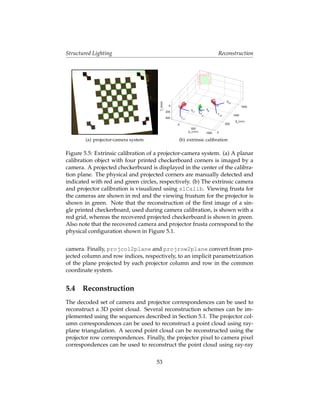
printed checkerboard corners. As shown in Figure 5.5, a single image of
the printed fiducials is used to recover the implicit equation of the calibra-
tion plane in the camera coordinate system. The 3D coordinate for each
projected checkerboard corner is then reconstructed. The 2D camera pixel
to 3D point correspondences are then used to estimate the intrinsic and
extrinsic calibration from multiple views of the planar calibration object.
A set of 20 example images of the projector calibration object are in-
cluded with the support code. In these examples, the printed fiducials were
horizontally separated by 406mm and vertically separated by 335mm. The
camera and projector calibration obtained using our procedure are also pro-
vided; note that the projector intrinsic and extrinsic parameters are in the
same format as camera calibration outputs from the Camera Calibration
Toolbox for M ATLAB. The provided m-file slCalib can be used to visual-
ize the calibration results.
A variety of Matlab utilities are provided to assist the reader in imple-
menting their own structured light scanner. The m-file campixel2ray
converts from camera pixel coordinates to an optical ray expressed in the
coordinate system of the first camera (if more than one camera is used). A
similar m-file projpixel2ray converts from projector pixel coordinates
to an optical ray expressed in the common coordinate system of the first
52](https://image.slidesharecdn.com/byo3d-090819162830-phpapp01/85/Build-Your-Own-3D-Scanner-Course-Notes-59-320.jpg)
![Surfaces from Point Clouds Merging Point Clouds
The SFL File Format
The SFL file format was introduced with Pointshop3D [ZPKG02] to pro-
vide a versatile file format to import and export point clouds with color,
normal vectors, and a radius per vertex describing the local sampling den-
sity. A SFL file is encoded in binary and features an extensible set of surfel
attributes, data compression, upward and downward compatibility, and
transparent conversion of surfel attributes, coordinate systems, and color
spaces. Pointshop3D is a software system for interactive editing of point-
based surfaces, developed at the Computer Graphics Lab at ETH Zurich.
6.1.2 Visualization
A well-established technique to render dense point clouds is point splat-
ting. Each point is regarded as an oriented disk in 3D, with the orientation
determined by the surface normal evaluated at each point, and the radius
of the disk usually stored as an additional parameter per vertex. As a re-
sult, each point is rendered as an ellipse. The color is determined by the
color stored with the point, the direction of the normal vector, and the illu-
mination model. The radii are chosen so that the ellipses overlap, resulting
in the perception of a continuous surface being rendered.
6.2 Merging Point Clouds
The triangulation-based 3D scanning methods described in previous chap-
ters are able to produce dense point clouds. However, due to visibility
constraints these point clouds may have large gaps without samples. In
order for a surface point to be reconstructed, it has to be illuminated by
a projector, and visible by a camera. In addition, the projected patterns
needs to illuminate the surface transversely for the camera to be able to
capture a sufficient amount of reflected light. In particular, only points on
the front-facing side of the object can be reconstructed (i.e., on the same side
as the projector and camera). Some methods to overcome these limitations
are discussed in Chapter 7. However, to produce a complete representa-
tion, multiple scans taken from various points of view must be integrated
to produce a point cloud with sufficient sampling density over the whole
visible surface of the object being scanned.
58](https://image.slidesharecdn.com/byo3d-090819162830-phpapp01/85/Build-Your-Own-3D-Scanner-Course-Notes-65-320.jpg)
![Surfaces from Point Clouds Surface Reconstruction from Point Clouds
where polygon faces are represented as loops of vertex coordinate vectors.
If two or more faces share a vertex, the vertex coordinates are repeated as
many times as needed. Another popular representation used in isosurface
algorithms is the IndexedFaceSet (IFS), describing polygon meshes with
simply-connected faces. In this representation the geometry is stored as ar-
rays of floating point numbers. In these notes we are primarily concerned
with the array coord of vertex coordinates, and to a lesser degree with the
array normal of face normals. The connectivity is described by the total
number V of vertices, and F faces, which are stored in the coordIndex
array as a sequence of loops of vertex indices, demarcated by values of −1.
6.3.3 Isosurfaces
An isosurface is a polygonal mesh surface representation produced by an
isosurface algorithm. An isosurface algorithm constructs a polygonal mesh
approximation of a smooth implicit surface S = {x : f (x) = 0} within
a bounded three-dimensional volume, from samples of a defining function
f (x) evaluated on the vertices of a volumetric grid. Marching Cubes [LC87]
and related algorithms operate on function values provided at the vertices
of hexahedral grids. Another family of isosurface algorithms operate on
functions evaluated at the vertices of tetrahedral grids [DK91]. Usually,
no additional information about the function is provided, and various in-
terpolation schemes are used to evaluate the function within grid cells, if
necessary. The most natural interpolation scheme for tetrahedral meshes is
linear interpolation, which we also adopt here.
6.3.4 Isosurface Construction Algorithms
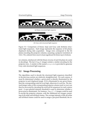
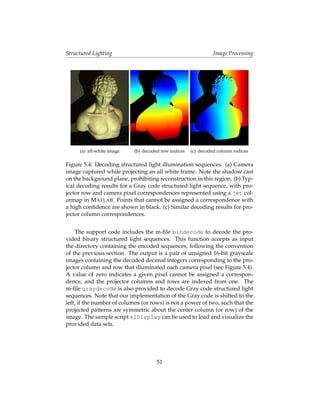
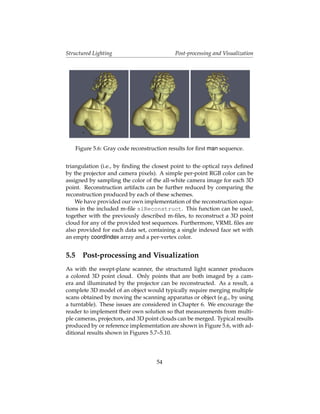
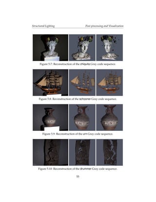
An isosurface algorithm producing a polygon soup output must solve three
key problems: (1) determining the quantity and location of isosurface ver-
tices within each cell, (2) determining how these vertices are connected
forming isosurface faces, and (3) determining globally consistent face ori-
entations. For isosurface algorithms producing IFS output, there is a fourth
problem to solve: identifying isosurface vertices lying on vertices and edges
of the volumetric grid. For many visualization applications, the polygon
soup representation is sufficient and acceptable, despite the storage over-
head. Isosurface vertices lying on vertices and edges of the volumetric grid
are independently generated multiple times. The main advantage of this
approach is that it is highly parallelizable. But, since most of these bound-
ary vertices are represented at least twice, it is not a compact representation.
63](https://image.slidesharecdn.com/byo3d-090819162830-phpapp01/85/Build-Your-Own-3D-Scanner-Course-Notes-70-320.jpg)
![Surfaces from Point Clouds Surface Reconstruction from Point Clouds
Figure 6.1: In isosurface algorithms, the sign of the function at the grid
vertices determines the topology and connectivity of the output polygonal
mesh within each tetrahedron. Mesh vertices are located on grid edges
where the function changes sign.
Researchers have proposed various solutions and design decisions (e.g.,
cell types, adaptive grids, topological complexity, interpolant order) to ad-
dress these four problems. The well-known Marching Cubes (MC) algo-
rithm uses a fixed hexahedral grid (i.e., cube cells) with linear interpolation
to find zero-crossings along the edges of the grid. These are the vertices of
the isosurface mesh. Second, polygonal faces are added connecting these
vertices using a table. The crucial observation made with MC is that the
possible connectivity of triangles in a cell can be computed independently
of the function samples and stored in a table. Out-of-core extensions, where
sequential layers of the volume are processed one at a time, are straightfor-
ward.
Similar tetrahedral-based algorithms [DK91, GH95, TPG99], dubbed
Marching Tetrahedra (MT), have also been developed (again using linear
interpolation). Although the cell is simpler, MT requires maintaining a
tetrahedral sampling grid. Out-of-core extensions require presorted traver-
sal schemes, such as in [CS97]. For an unsorted tetrahedral grid, hash tables
are used to save and retrieve vertices lying on edges of the volumetric grid.
As an example of an isosurface algorithm, we discuss MT in more detail.
Marching Tetrahedra
MT operates on the following input data: (1) a tetrahedral grid and (2)
one piecewise linear function f (x), defined by its values at the grid ver-
tices. Within the tetrahedron with vertices x0 , x1 , x2 , x3 ∈ IR3 , the func-
64](https://image.slidesharecdn.com/byo3d-090819162830-phpapp01/85/Build-Your-Own-3D-Scanner-Course-Notes-71-320.jpg)
![Surfaces from Point Clouds Surface Reconstruction from Point Clouds
i (i3 i2 i1 i0 ) face
0 0000 [-1]
1 0001 [2,1,0,-1]
2 0010 [0,3,4,-1]
3 0011 [1,3,4,2,-1]
4 0100 [1,5,3,-1] e edge
5 0101 [0,2,5,3,-1] 0 (0,1)
6 0110 [0,3,5,4,-1] 1 (0,2)
7 0111 [1,5,2,-1] 2 (0,3)
8 1000 [2,5,1,-1] 3 (1,2)
9 1001 [4,5,3,0,-1] 4 (1,3)
10 1010 [3,5,2,0,-1] 5 (2,3)
11 1011 [3,5,1,-1]
12 1100 [2,4,3,1,-1]
13 1101 [4,3,0,-1]
14 1110 [0,1,2,-1]
15 1111 [-1]
Table 6.1: Look-up tables for tetrahedral mesh isosurface evaluation. Note
that consistent face orientation is encoded within the table. Indices stored
in the first table reference tetrahedron edges, as indicated by the second
table of vertex pairs (and further illustrated in Figure 6.1). In this case,
only edge indices {1, 2, 3, 4} have associated isosurface vertex coordinates,
which are shared with neighboring cells.
tion is linear and can be described in terms of the barycentric coordinates
b = (b0 , b1 , b2 , b3 )t of an arbitrary internal point x = b0 x0 +b1 x1 +b2 x2 +b3 x3
with respect to the four vertices: f (x) = b0 f (x0 ) + b1 f (x1 ) + b2 f (x2 ) +
b3 f (x3 ), where b0 , b1 , b2 , b3 ≥ 0 and b0 + b1 + b2 + b3 = 1. As illustrated in
Figure 6.1, the sign of the function at the four grid vertices determines the
connectivity (e.g., triangle, quadrilateral, or empty) of the output polygo-
nal mesh within each tetrahedron. There are actually 16 = 24 cases, which
modulo symmetries and sign changes reduce to only three. Each grid edge,
whose end vertex values change sign, corresponds to an isosurface mesh
vertex. The exact location of the vertex along the edge is determined by
linear interpolation from the actual function values, but note that the 16
cases can be precomputed and stored in a table indexed by a 4-bit integer
i = (i3 i2 i1 i0 ), where ij = 1 if f (xj ) > 0 and ij = 0, if f (xj ) < 0. The full
table is shown in Table 6.1. The cases f (xj ) = 0 are singular and require
special treatment. For example, the index is i = (0100) = 4 for Figure 6.1(a),
65](https://image.slidesharecdn.com/byo3d-090819162830-phpapp01/85/Build-Your-Own-3D-Scanner-Course-Notes-72-320.jpg)
![Surfaces from Point Clouds Surface Reconstruction from Point Clouds
and i = (1100) = 12 for Figure 6.1(b). Orientation for the isosurface faces,
consistent with the orientation of the containing tetrahedron, can be ob-
tained from connectivity alone (and are encoded in the look-up table as
shown in Table 6.1). For IFS output it is also necessary to stitch vertices as
described above.
Algorithms to polygonize implicit surfaces [Blo88], where the implicit
functions are provided in analytic form, are closely related to isosurface
algorithms. For example, Bloomenthal and Ferguson [BF95] extract non-
manifold isosurfaces produced from trimming implicits and parameter-
ics using a tetrahedral isosurface algorithm. [WvO96] polygonize boolean
combinations of skeletal implicits (Boolean Compound Soft Objects), ap-
plying an iterative solver and face subdivision for placing vertices along
feature edges and points. Suffern and Balsys [SB03] present an algorithm
to polygonize surfaces defined by two implicit functions provided in ana-
lytic form; this same algorithm can compute bi-iso-lines of pairs of implicits
for rendering.
Isosurface Algorithms on Hexahedral Grids
An isosurface algorithm constructs a polygon mesh approximation of a
level set of a scalar function defined in a finite 3D volume. The function
f (p) is usually specified by its values fα = f (pα ) on a regular grid of three
dimensional points
G = {pα : α = (α0 , α1 , α2 ) ∈ [[n0 ]]×[[n1 ]]×[[n2 ]]} ,
where [[nj ]] = {0, . . . , nj − 1}, and by a method to interpolate in between
these values. The surface is usually represented as a polygon mesh, and
is specified by its isovalue f0 . Furthermore, the interpolation scheme is as-
sumed to be linear along the edges of the grid, so that the isosurface cuts
each edge in no more than one point. If pα and pβ are grid points con-
nected by an edge, and fα > f0 > fβ , the location of the point pαβ where
the isosurface intersects the edge is
fα − f0 fβ − f0
pαβ = pβ + pα . (6.3)
fα − fβ fβ − fα
Marching Cubes
One of the most popular isosurface extraction algorithms is Marching Cubes
[LC87]. In this algorithm the points defined by the intersection of the iso-
surface with the edges of the grid are the vertices of the polygon mesh.
66](https://image.slidesharecdn.com/byo3d-090819162830-phpapp01/85/Build-Your-Own-3D-Scanner-Course-Notes-73-320.jpg)
![Surfaces from Point Clouds Surface Reconstruction from Point Clouds
These vertices are connected forming polygon faces according to the fol-
lowing procedure. Each set of eight neighboring grid points define a small
cube called a cell
Cα = {pα+β : β ∈ {0, 1}3 }.
Since the function value associated with each of the eight corners of a cell
may be either above or below the isovalue (isovalues equal to grid function
values are called singular and should be avoided), there are 28 = 256 pos-
sible configurations. A polygonization of the vertices within each cell, for
each one of these configurations, is stored in a static look-up table. When
symmetries are taken into account, the size of the table can be reduced sig-
nificantly.
6.3.5 Algorithms to Fit Implicit Surfaces to Point Clouds
Let U be a relatively open and simply-connected subset of IR3 , and f : U →
IR a smooth function. The gradient f is a vector field defined on U . Given
an oriented point cloud, i.e., a finite set D of point-vector pairs (p, n), where p
is an interior point of U , and n is a unit length 3D vector, the problem is to
find a smooth function f so that f (p) ≈ 0 and (p) ≈ n for every oriented
point (p, n) in the data set D. We call the zero iso-level set of such a function
{p : f (p) = 0} a surface fit, or surface reconstruction, for the data set D.
We are particularly interested in fitting isosurfaces to oriented point
points. For the sake of simplicity, we assume that the domain is the unit
cube U = [0, 1]3 , the typical domain of an isosurface defined on an hexa-
hedral mesh, and the isolevel is zero, i.e., the isosurface to be fitted to the
data points is {p : f (p) = 0}, but of course, the argument applies in more
general cases.
Figure 6.2: Early results of Vector Field Isosurface reconstruction from oriented
point clouds introduced in [ST05].
Figure 6.2 shows results of surface reconstruction from an oriented point
cloud using the simple variational formulation presented in [ST05], where
oriented data points are regarded as samples of the gradient vector field of
67](https://image.slidesharecdn.com/byo3d-090819162830-phpapp01/85/Build-Your-Own-3D-Scanner-Course-Notes-74-320.jpg)
![Surfaces from Point Clouds Surface Reconstruction from Point Clouds
an implicit function, which is estimated by minimizing this energy function
m m
2 2 2
E1 (f ) = f (pi ) + λ1 f (pi ) − ni + λ2 Hf (x) dx , (6.4)
i=1 i=1 V
where f (x) is the implicit function being estimated, f (x) is the gradient of
f , Hf (x) is the Hessian of f (x), (p1 , n1 ), . . . , (pm , nm ) are point-normal data
pairs, V is a bounding volume, and λ1 and λ2 are regularization parame-
ters. Minimizing this energy requires the solution of a simple large and
sparse least squares problem. The result is usually unique modulo an addi-
tive constant. Given that, for rendering or post-processing, isosurfaces are
extracted from scalar functions defined over regular grids (e.g., via March-
ing Cubes), it is worth exploring representations of implicit functions de-
fined as a regular scalar fields. Finite difference discretization is used in
[ST05], with the volume integral resulting in a sum of gradient differences
over the edges of the regular grid, yet Equation 6.4 can be discretized in
many other ways.
68](https://image.slidesharecdn.com/byo3d-090819162830-phpapp01/85/Build-Your-Own-3D-Scanner-Course-Notes-75-320.jpg)
![Applications and Emerging Trends Extensions
7.1.1 3D Slit Scanning with Planar Constraints
Leotta et al. [LVT08] propose “3D slit scanning with planar constraints” as a
novel 3D point reconstruction algorithm for multi-view swept-plane scan-
ners. A planarity constraint is proposed, based on the fact that all observed
points on a projected stripe must lie on the same 3D plane. The plane lin-
early parameterizes a homography [HZ04] between any pair of images of
the laser stripe, which can be recovered from point correspondences de-
rived from epipolar geometry [SCD∗ 06]. This planarity constraint reduces
reconstruction outliers and allows for the reconstruction of points seen in
only one view.
As shown in Figure 7.1, a catadioptric stereo rig is constructed to re-
move artifacts from camera synchronization errors and non-uniform pro-
jection. The same physical setup was originally suggested by Davis and
Chen [DC01]. It maintains many of the desirable traits of other laser range
scanners while eliminating several actuated components (e.g., the trans-
lation and rotation stages in Figure 1.2), thereby reducing calibration com-
plexity and increasing maintainability and scan repeatability. Tracing back-
ward from the camera, the optical rays first encounter a pair of primary
mirrors forming a “V” shape. The rays from the left half of the image are
reflected to the left, and those from the right half are reflected to the right.
Next, the rays on each side encounter a secondary mirror that reflects them
back toward the center and forward. The viewing volumes of the left and
right sides of the image intersect near the target object. Each half of the
resulting image may be considered as a separate camera for image process-
ing. The standard camera calibration techniques for determining camera
position and orientation still apply to each half.
Similar to Chapter 4, a user scans an object by manually manipulating
a hand-held laser line projector. Visual feedback is provided at interactive
rates in the form of incremental 3D reconstructions, allowing the user to
sweep the line across any unscanned regions. Once the plane of light has
been estimated, there are several ways to reconstruct the 3D location of
the points. First, consider the non-singular case when a unique plane of
light can be determined. If a point is visible from only one camera (due to
occlusion or indeterminate correspondence), it can still be reconstructed by
ray-plane intersection. For points visible in both views, it is beneficial to use
the data from both views. One approach is to triangulate the points using
ray-ray intersection. This is the approach taken by Davis and Chen [DC01].
While both views are used, the constraint that the resulting 3D point lies
on the laser stripe plane is not strictly enforced.
70](https://image.slidesharecdn.com/byo3d-090819162830-phpapp01/85/Build-Your-Own-3D-Scanner-Course-Notes-77-320.jpg)
![Applications and Emerging Trends Extensions
Figure 7.1: 3D slit scanning with planar constraints. (Top left) The catadiop-
tric scanning rig. (Top right) A sample image. (Bottom left) Diagram of the
scanning system. Note that the camera captures a stereo image, each half
originating from a virtual camera produced by mirror reflection. (Bottom
right) Working volume and scannable surfaces of a T-shaped object. Note
that the working volume is the union of the virtual camera pair, excluding
occluded regions. (Figure from [LVT08].)
Leotta et al. [LVT08] examine how such a planarity constraint can en-
hance the reconstruction. Their first approach involves triangulating a point
(using ray-ray intersection) and then projecting it onto the closest point on
the corresponding 3D laser plane. While such an approach combines the
stability of triangulation with the constraint of planarity, there is no guar-
antee that the projected point is the optimal location on the plane. In their
second approach, they compute an optimal triangulation constrained to the
plane. The two projection approaches are compared in Figure 7.2. We refer
the reader to the paper for additional technical details on the derivation of
the optimally projected point. Illustrative results are shown in Figure 7.3.
Note the benefit of adding points seen in only one view, as well as the result
of applying optimal planar projection.
71](https://image.slidesharecdn.com/byo3d-090819162830-phpapp01/85/Build-Your-Own-3D-Scanner-Course-Notes-78-320.jpg)
![Applications and Emerging Trends Extensions
(a) laser plane to image homographies (b) projection onto the laser plane
Figure 7.2: (a) Homographies between the laser plane and image planes.
(b) A 2D view of triangulation and both orthogonal and optimal projection
onto the laser plane. (Figure from [LVT08].)
(a) catadioptric stereo view (b) triangulated (c) optimal (d) all points
Figure 7.3: Reconstruction results. The catadioptric image (a) and output
point clouds using triangulation (b) and optimal planar projection (c). Note
that points in (c) are reconstructed from both views, whereas (d) shows the
additional of points seen from only one view. (Figure from [LVT08].)
72](https://image.slidesharecdn.com/byo3d-090819162830-phpapp01/85/Build-Your-Own-3D-Scanner-Course-Notes-79-320.jpg)
![Applications and Emerging Trends Extensions
7.1.2 Surround Structured Lighting
Lanman et al. [LCT07] propose “surround structured lighting” as a novel
modification of a traditional single projector-camera structured light sys-
tem that allows full 360◦ surface reconstructions, without requiring turnta-
bles or multiple scans. As shown in Figure 7.4, the basic concept is to il-
luminate the object from all directions with a structured pattern consisting
of horizontal planes of light, while imaging the object from multiple views
using a single camera and mirrors. A key benefit of this design is to ensure
that each point on the object surface can be assigned an unambiguous Gray
code sequence, despite the possibility of being illuminated from multiple
directions.
Traditional structured light projectors, for example those using Gray
code sequences, cannot be used to simultaneously illuminate an object from
all sides (using more than one projector) due to interference. If such a con-
figuration was used, then there is a high probability that certain points
would be illuminated by multiple projectors. In such circumstances, multi-
ple Gray codes would interfere, resulting in erroneous reconstruction due
to decoding errors. Rather than using multiple projectors (each with a sin-
gle center of projection), the proposed “surround structured lighting” sys-
tem uses a single orthographic projector and a pair of planar mirrors.
As shown from above and in profile in Figure 7.4, the key components
of the proposed scanning system are an orthographic projector, two pla-
nar mirrors aligned such that their normal vectors are contained within the
plane of light created by each projector row, and a single high-resolution
digital camera. If any structured light pattern consisting of horizontal bi-
nary stripes is implemented, then the object can be fully illuminated on all
sides due to direct and reflected projected light. Furthermore, if the cam-
era’s field of view contains the object and both mirrors, then it will record
five views of the illuminated object: one direct view, two first reflections,
and two second reflections [FNdJV06]. By carefully aligning the mirrors so
that individual projector rows are always reflected back upon themselves,
only a single Gray code sequence will be assigned to each projector row—
ensuring each vertically-space plane in the reconstruction volume receives
a unique code. The full structured light pattern combined with the five
views (see Figure 7.5) provides sufficient information for a nearly complete
surface reconstruction from a single camera position, following methods
similar to those in Chapter 5.
The required orthographic projector can be implemented using a stan-
dard off-the-shelf DLP projector and a Fresnel lens, similar to that used by
73](https://image.slidesharecdn.com/byo3d-090819162830-phpapp01/85/Build-Your-Own-3D-Scanner-Course-Notes-80-320.jpg)
![Applications and Emerging Trends Extensions
c12 c21
v12 v21
v1 v2
M1 M2 c2
c1
v0
c0
Figure 7.4: Surround structured lighting for full object scanning. (Top left)
Surround structured lighting prototype. (Top right) The position of the
real c0 and virtual {c1 , c2 , c12 , c21 } cameras with respect to mirrors {M1 ,
M2 }. (Middle) After reflection, multiple rays from a single projector row
illuminate the object from all sides while remaining co-planar. (Bottom)
Prototype, from left to right: the first-surface planar mirrors, Fresnel lens,
high-resolution digital camera, and DLP projector. (Figure from [LCT07].)
74](https://image.slidesharecdn.com/byo3d-090819162830-phpapp01/85/Build-Your-Own-3D-Scanner-Course-Notes-81-320.jpg)
![Applications and Emerging Trends Extensions
Figure 7.5: Example of an orthographic Gray code pattern and recovered
projector rows. (Top left) Scene, as viewed under ambient illumination, for
use in texture mapping. (Top right) Per-pixel projector row indices recov-
ered by decoding the projected Gray code sequence (shaded by increasing
index, from red to blue). (Bottom left) Fourth projected Gray code. (Bottom
right) Sixth projected Gray code. (Figure from [LCT07].)
Nayar and Anand [NA06] for volumetric display. The Fresnel lens converts
light rays diverging from the focal point to parallel rays and can be man-
ufactured in large sizes, while remaining lightweight and inexpensive. Al-
though the projector can be modeled as a pinhole projector (see Chapters 2
and 3), practically it will have a finite aperture lens and a corresponding
finite depth of field. This makes conversion to a perfectly-orthographic set
of rays impossible with the Fresnel lens, yet an acceptable approximation
is still feasible.
The planar mirrors are positioned, following Forbes et al. [FNdJV06],
75](https://image.slidesharecdn.com/byo3d-090819162830-phpapp01/85/Build-Your-Own-3D-Scanner-Course-Notes-82-320.jpg)
![Applications and Emerging Trends Extensions
Figure 7.6: Summary of reconstruction results. From left to right: the input
images used for texture mapping and four views of the 3-D point cloud re-
covered using the proposed method with a single camera and orthographic
projector. (Figure from [LCT07].)
such that their surface normals are roughly 72◦ apart and perpendicular to
the projected planes of light. This ensures that five equally-spaced views
are created. The mirrors are mounted on gimbals with fine tuning knobs
in order to facilitate precise positioning. Furthermore, first-surface mirrors
are used to eliminate refraction from the protective layer of glass covering
the reflective surface in lower-cost second-surface mirrors (e.g., those one
would typically buy at a hardware store).
Because of the unique design of the scanning system, calibration of
the multiple components is a non-trivial task. Lanman et al. [LCT07] ad-
dress these issues by developing customized calibration procedures di-
vided across three stages: (1) configuration of the orthographic projector,
(2) alignment of the planar mirrors, and (3) calibration of the camera/mirror
system. Key results include the use of Gray codes and homographies to cal-
ibrate the orthographic imaging system, procedures to ensure precise me-
chanical alignment of the scanning apparatus, and optimization techniques
for calibrating catadioptic systems containing a single digital camera and
one or more planar mirrors. We refer readers to the paper for additional
calibration details.
76](https://image.slidesharecdn.com/byo3d-090819162830-phpapp01/85/Build-Your-Own-3D-Scanner-Course-Notes-83-320.jpg)
![Applications and Emerging Trends Recent Advances and Further Reading
Reconstruction proceeds in a similar manner to that used in conven-
tional structured light scanners. A key modification, however, is the re-
quirement that each of the five sub-images must be assigned to a specific
real or virtual camera. Afterwards, each optical ray is intersected with its
associated projector plane (corresponding to an individual orthographic
projector row) in order to reconstruct a dense 3-D point cloud. Illustrative
results are tabulated in Figure 7.6.
While the current prototype can only scan relatively small volumes,
this system has already demonstrated practical benefits for telecollabora-
tion applications, allowing for rapid acquisition of nearly complete object
models. We hope the reader is inspired to pursue similar non-traditional
optical configurations using their own 3D scanners. To this end, we also
recommend reviewing related work by Epstein et al. [EGPP04], on incor-
porating planar mirrors with structured lighting, as well as the work of
Nayar and Anand [NA06] on creating orthographic projectors using simi-
lar configurations of Fresnel lenses.
7.2 Recent Advances and Further Reading
3D scanning remains a very active area of computer graphics and vision
research. While numerous commercial products are available, few achieve
the ease of use, visual fidelity, and reliability of simple point-and-shoot
cameras. As briefly reviewed in Chapter 1, a myriad collection of both
passive and active non-contact optical metrology methods have emerged.
Many have not withstood the test of time, yielding to more flexible, lower-
cost alternatives. Some, like 3D slit scanning and structured lighting, have
become widespread—in equal parts due to their performance, as well as
their conceptual and practical accessibility.
In this section we briefly review late-breaking work and other advances
that are shaping the field of optical 3D scanning. Before continuing, we
encourage the reader to consider the materials from closely-related SIG-
GRAPH 2009 courses. Heidrich and Ihrke present Acquisition of Optically
Complex Objects and Phenomena, discussing methods to scan problematic ob-
jects with translucent and specular materials. In a similar vein, Narasimhan
et al. present Scattering, a course on imaging through participating me-
dia. Several additional courses focus on specialized scanning applications;
Debevec et al. cover face scanning in The Digital Emily Project: Photoreal
Facial Modeling and Animation, whereas Cain et al. discuss scanning appli-
cations in archeology and art history in Computation & Cultural Heritage:
77](https://image.slidesharecdn.com/byo3d-090819162830-phpapp01/85/Build-Your-Own-3D-Scanner-Course-Notes-84-320.jpg)
![Applications and Emerging Trends Recent Advances and Further Reading
Fundamentals and Applications. Finally, we recommend Gross’ Point Based
Graphics-State of the Art and Recent Advances for a further tutorial on point-
based rendering.
Applying 3D scanning in practical situations requires carefully consid-
ering the complexities of the object you are measuring. These complex-
ities are explored, to great detail, by two pioneering efforts: the Digital
Michelangelo Project [LPC∗ 00] and the Piet` Project [BRM∗ 02]. In the for-
a
mer, the subsurface scattering properties of marble were considered; in the
later, lightweight commercial laser scanners and photometric stereo were
deployed to create a portable solution. Building low-cost, reliable systems
for rapidly scanning such complex objects remains a challenging task.
Passive methods continue to evolve. Light fields [LH96, GGSC96], cap-
tured using either camera arrays [WJV∗ 05] or specialized plenoptic cam-
eras [AW92, NLB∗ 05, VRA∗ 07], record the spatial and angular variation of
the irradiance passing between two planes in the world (assuming no at-
tenuation within the medium). Vaish et al. [VLS∗ 06] recover depth maps
from light fields. Such imagery can be used to synthesize a virtual focal
stack, allowing the method of Nayar and Nakagawa [NN94] to estimate
shape-from-focus. Lanman et al. [LRAT08] extend light field capture to al-
low single-shot visual hull reconstruction of opaque objects.
The limitations of most active scanning methods are well-known. Specif-
ically, scanning diffuse surfaces is straightforward; however, scenes that
contain translucence, subsurface scattering, or strong reflections lead to
artifacts and often require additional measures to be taken—often involv-
ing dappling the surface with certain Lambertian powders. Scanning such
hard-to-scan items has received significant attenuation over the last few
years. Hullin et al. [HFI∗ 08] immerse transparent objects in a florescent liq-
uid. This liquid creates an inverse image as that produced by a traditional
3D slit scanner, where the laser sheet is visible up to the point of contact.
In a similar vein, tomographic methods are used to reconstruct transparent
objects; first, by immersion in an index-matching liquid [TBH06], and sec-
ond through the use of background-oriented Schlieren imaging [AIH∗ 08].
In addition to scanning objects with complex material properties, ac-
tive imaging is beginning to be applied to challenging environments with
anisotropic participating media. For example, in typical underwater imag-
ing conditions, visible light is strongly scattered by suspended particu-
lates. Narasimhan et al. consider laser striping and photometric stereo in
underwater imaging [NN05], as well as structured light in scattering me-
dia [NNSK08]. Such challenging environments represent the next horizon
for active 3D imaging.
78](https://image.slidesharecdn.com/byo3d-090819162830-phpapp01/85/Build-Your-Own-3D-Scanner-Course-Notes-85-320.jpg)

![Bibliography
[AIH∗ 08] ATCHESON B., I HRKE I., H EIDRICH W., T EVS A., B RADLEY
D., M AGNOR M., S EIDEL H.-P.: Time-resolved 3d capture of
non-stationary gas flows. ACM Transactions on Graphics (Proc.
SIGGRAPH Asia) 27, 5 (2008), 132. 78
[AW92] A DELSON T., WANG J.: Single lens stereo with a plenoptic
camera. IEEE TPAMI 2, 14 (1992), 99–106. 78
[BF95] B LOOMENTHAL J., F ERGUSON K.: Polygonization of non-
manifold implicit surfaces. In SIGGRAPH ’95: ACM SIG-
GRAPH 1995 papers (1995), pp. 309–316. 66
[BK08] B RADSKI G., K AEHLER A.: Learning OpenCV: Computer Vision
with the OpenCV Library. O’Reilly Media, Inc., 2008. 32
[Bla04] B LAIS F.: Review of 20 years of range sensor development.
Journal of Electronic Imaging 13, 1 (2004), 231–240. 5
[Blo88] B LOOMENTHAL J.: Polygonization of Implicit Surfaces. Com-
puter Aided Geometric Design 5, 4 (1988), 341–355. 66
[Bou] B OUGUET J.-Y.: Camera calibration toolbox for matlab. http:
//www.vision.caltech.edu/bouguetj/calib_doc/.
28, 40, 52
[Bou99] B OUGUET J.-Y.: Visual methods for three-dimensional modeling.
PhD thesis, California Institute of Technology, 1999. 38, 42
[BP] B OUGUET J.-Y., P ERONA P.: 3d photography on your
desk. http://www.vision.caltech.edu/bouguetj/
ICCV98/. 7, 35, 36, 45
80](https://image.slidesharecdn.com/byo3d-090819162830-phpapp01/85/Build-Your-Own-3D-Scanner-Course-Notes-87-320.jpg)
![Bibliography
[BP99] B OUGUET J.-Y., P ERONA P.: 3d photography using shadows
in dual-space geometry. Int. J. Comput. Vision 35, 2 (1999), 129–
149. 35, 38, 39, 42
[BRM∗ 02] B ERNARDINI F., R USHMEIER H., M ARTIN I. M., M ITTLEMAN
J., TAUBIN G.: Building a digital model of michelangelo’s
florentine piet` . IEEE Computer Graphics and Applications 22
a
(2002), 59–67. 78
[CG00] C IPOLLA R., G IBLIN P.: Visual Motion of Curves and Surfaces.
Cambridge University Press, 2000. 4
[CMU] CMU IEEE 1394 digital camera driver, version 6.4.5.
http://www.cs.cmu.edu/ iwan/1394/. 25
[Cre] C REAFORM: Handyscan 3D. http://www.creaform3d.
com/en/handyscan3d/products/exascan.aspx. 6
[CS97] C HIANG Y., S ILVA C. T.: I/O Optimal Isosurface Extraction. In
IEEE Visualization 1997, Conference Proceedings (1997), pp. 293–
300. 64
[CTMS03] C ARRANZA J., T HEOBALT C., M AGNOR M. A., S EIDEL H.-P.:
Free-viewpoint video of human actors. ACM Trans. Graph. 22,
3 (2003), 569–577. 4
[dAST∗ 08] DE A GUIAR E., S TOLL C., T HEOBALT C., A HMED N., S EIDEL
H.-P., T HRUN S.: Performance capture from sparse multi-view
video. In SIGGRAPH ’08: ACM SIGGRAPH 2008 papers (2008),
pp. 1–10. 4
[DC01] D AVIS J., C HEN X.: A laser range scanner designed for mini-
mum calibration complexity. In Proceedings of the International
Conference on 3-D Digital Imaging and Modeling (3DIM) (2001),
p. 91. 70
[Deb97] D EBEVEC P. E.: Facade: modeling and rendering architecture
from photographs and the campanile model. In SIGGRAPH
’97: ACM SIGGRAPH 97 Visual Proceedings (1997), p. 254. 4
[DK91] D OI A., K OIDE A.: An Efficient Method of Triangulating
Equivalued Surfaces by Using Tetrahedral Cells. IEICE Transac-
tions on Communications and Electronics Information Systems E74,
1 (Jan. 1991), 214–224. 63, 64
81](https://image.slidesharecdn.com/byo3d-090819162830-phpapp01/85/Build-Your-Own-3D-Scanner-Course-Notes-88-320.jpg)
![Bibliography
[Edm] E DMUND O PTICS:. http://www.edmundoptics.com. 37
[EGPP04] ´
E PSTEIN E., G RANGER -P ICH E M., P OULIN P.: Exploiting mir-
rors in interactive reconstruction with structured light. In Vi-
sion, Modeling, and Visualization 2004 (2004), pp. 125–132. 77
[Far97] FARID H.: Range Estimation by Optical Differentiation. PhD the-
sis, University of Pennsylvania, 1997. 4
[FNdJV06] F ORBES K., N ICOLLS F., DE J AGER G., V OIGT A.: Shape-from-
silhouette with two mirrors and an uncalibrated camera. In
ECCV 2006 (2006), pp. 165–178. 73, 75
[FWM98] F ERRYMAN J. M., W ORRALL A. D., M AYBANK S. J.: Learn-
ing enhanced 3d models for vehicle tracking. In BMVC (1998),
pp. 873–882. 4
[GGSC96] G ORTLER S. J., G RZESZCZUK R., S ZELISKI R., C OHEN M. F.:
The lumigraph. In SIGGRAPH ’96: ACM SIGGRAPH 1996 pa-
pers (1996), pp. 43–54. 78
[GH95] ´
G U E ZIEC A., H UMMEL R.: Exploiting Triangulated Surface
Extraction Using Tetrahedral Decomposition. IEEE Transac-
tions on Visualization and Computer Graphics 1, 4 (1995). 64
[GSP06] G REENGARD A., S CHECHNER Y. Y., P IESTUN R.: Depth from
diffracted rotation. Opt. Lett. 31, 2 (2006), 181–183. 4
[HARN06] H SU S., A CHARYA S., R AFII A., N EW R.: Performance of a
time-of-flight range camera for intelligent vehicle safety ap-
plications. Advanced Microsystems for Automotive Applications
(2006). 6
[Hec01] H ECHT E.: Optics (4th Edition). Addison Wesley, 2001. 4
[HFI∗ 08] H ULLIN M. B., F UCHS M., I HRKE I., S EIDEL H.-P., L ENSCH
H. P. A.: Fluorescent immersion range scanning. ACM Trans.
Graph. 27, 3 (2008), 1–10. 78
[HVB∗ 07] ´
H ERN ANDEZ C., V OGIATZIS G., B ROSTOW G. J., S TENGER B.,
C IPOLLA R.: Non-rigid photometric stereo with colored lights.
In Proc. of the 11th IEEE Intl. Conf. on Comp. Vision (ICCV) (2007).
7
82](https://image.slidesharecdn.com/byo3d-090819162830-phpapp01/85/Build-Your-Own-3D-Scanner-Course-Notes-89-320.jpg)
![Bibliography
[HZ04] H ARTLEY R. I., Z ISSERMAN A.: Multiple View Geometry in Com-
puter Vision, second ed. Cambridge University Press, 2004. 3,
26, 70
[ISM84] I NOKUCHI S., S ATO K., M ATSUDA F.: Range imaging system
for 3-d object recognition. In Proceedings of the International Con-
ference on Pattern Recognition (1984), pp. 806–808. 48
[IY01] I DDAN G. J., YAHAV G.: Three-dimensional imaging in the
studio and elsewhere. Three-Dimensional Image Capture and Ap-
plications IV 4298, 1 (2001), 48–55. 6
[KM00] K AKADIARIS I., M ETAXAS D.: Model-based estimation of 3d
human motion. IEEE Transactions on Pattern Analysis and Ma-
chine Intelligence 22, 12 (2000), 1453–1459. 4
[Las] L ASER D ESIGN I NC .: Surveyor DT-2000 desktop 3D
laser scanner. http://www.laserdesign.com/
quick-attachments/hardware/low-res/dt-series.
pdf. 6
[Lau94] L AURENTINI A.: The Visual Hull Concept for Silhouette-Based
Image Understanding. IEEE TPAMI 16, 2 (1994), 150–162. 3
[LC87] L ORENSEN W. L., C LINE H. E.: Marching Cubes: A High
Resolution 3D Surface Construction Algorithm. In Siggraph’87,
Conference Proceedings (1987), ACM Press, pp. 163–169. 63, 66
[LCT07] L ANMAN D., C RISPELL D., TAUBIN G.: Surround structured
lighting for full object scanning. In Proceedings of the Interna-
tional Conference on 3-D Digital Imaging and Modeling (3DIM)
(2007), pp. 107–116. 73, 74, 75, 76
[LFDF07] L EVIN A., F ERGUS R., D URAND F., F REEMAN W. T.: Image
and depth from a conventional camera with a coded aperture.
ACM Trans. Graph. 26, 3 (2007), 70. 4
[LH96] L EVOY M., H ANRAHAN P.: Light field rendering. In Proc. of
ACM SIGGRAPH (1996), pp. 31–42. 78
[LN04] L AND M. F., N ILSSON D.-E.: Animal Eyes. Oxford University
Press, 2004. 2
83](https://image.slidesharecdn.com/byo3d-090819162830-phpapp01/85/Build-Your-Own-3D-Scanner-Course-Notes-90-320.jpg)
![Bibliography
[LPC∗ 00] L EVOY M., P ULLI K., C URLESS B., R USINKIEWICZ S., K OLLER
D., P EREIRA L., G INZTON M., A NDERSON S., D AVIS J., G INS -
BERG J., S HADE J., F ULK D.: The digital michelangelo project:
3D scanning of large statues. In Proceedings of ACM SIGGRAPH
2000 (2000), pp. 131–144. 78
[LRAT08] L ANMAN D., R ASKAR R., A GRAWAL A., TAUBIN G.: Shield
fields: modeling and capturing 3d occluders. ACM Trans.
Graph. 27, 5 (2008), 1–10. 78
[LT] L ANMAN D., TAUBIN G.: Build your own 3d scanner: 3d
photography for beginners (course website). http://mesh.
brown.edu/dlanman/scan3d. 37
[LVT08] L EOTTA M. J., VANDERGON A., TAUBIN G.: 3d slit scanning
with planar constraints. Computer Graphics Forum 27, 8 (Dec.
2008), 2066–2080. 70, 71, 72
[Mat] M ATH W ORKS , I NC: Image acquisition toolbox. http://www.
mathworks.com/products/imaq/. 25, 46
[MBR∗ 00] M ATUSIK W., B UEHLER C., R ASKAR R., G ORTLER S. J.,
M C M ILLAN L.: Image-based visual hulls. In SIGGRAPH ’00:
ACM SIGGRAPH 2000 papers (2000), pp. 369–374. 4
[Mit] M ITSUBISHI E LECTRIC C ORP.: XD300U user man-
ual. http://www.projectorcentral.com/pdf/
projector_manual_1921.pdf. 46
[MPL04] M ARC R. Y., P OLLEFEYS M., L I S.: Improved real-time stereo
on commodity graphics hardware. In In IEEE Workshop on Real-
time 3D Sensors and Their Use (2004). 3
[MSKS05] M A Y., S OATTO S., K OSECKA J., S ASTRY S. S.: An Invitation to
3-D Vision. Springer, 2005. 26, 39
[NA06] N AYAR S. K., A NAND V.: Projection Volumetric Display Using
Passive Optical Scatterers. Tech. rep., July 2006. 75, 77
[Nex] N EXT E NGINE: 3D Scanner HD. https://www.
nextengine.com/indexSecure.htm. 6
[NLB∗ 05] N G R., L EVOY M., B REDIF M., D UVAL G., H OROWITZ M.,
H ANRAHAN P.: Light field photography with a hand-held
plenoptic camera. Tech Report, Stanford University (2005). 78
84](https://image.slidesharecdn.com/byo3d-090819162830-phpapp01/85/Build-Your-Own-3D-Scanner-Course-Notes-91-320.jpg)
![Bibliography
[NN94] N AYAR S. K., N AKAGAWA Y.: Shape from focus. IEEE Trans.
Pattern Anal. Mach. Intell. 16, 8 (1994), 824–831. 4, 78
[NN05] N ARASIMHAN S. G., N AYAR S.: Structured light methods for
underwater imaging: light stripe scanning and photometric
stereo. In Proceedings of 2005 MTS/IEEE OCEANS (September
2005), vol. 3, pp. 2610 – 2617. 78
[NNSK08] N ARASIMHAN S. G., N AYAR S. K., S UN B., K OPPAL S. J.:
Structured light in scattering media. In SIGGRAPH Asia ’08:
ACM SIGGRAPH Asia 2008 courses (2008), pp. 1–8. 78
[Opea] Open source computer vision library. http://
sourceforge.net/projects/opencvlibrary/. 26,
40
[Opeb] OpenCV wiki. http://opencv.willowgarage.com/
wiki/. 46
[OSS∗ 00] O RMONEIT D., S IDENBLADH H., S IDENBLADH H., B LACK
M. J., H ASTIE T., F LEET D. J.: Learning and tracking human
motion using functional analysis. In IEEE Workshop on Human
Modeling, Analysis and Synthesis (2000), pp. 2–9. 4
[PA82] P OSDAMER J., A LTSCHULER M.: Surface measurement by
space encoded projected beam systems. Computer Graphics and
Image Processing 18 (1982), 1–17. 47
[Poia] P OINT G REY R ESEARCH , I NC .: Grasshopper IEEE-1394b
digital camera. http://www.ptgrey.com/products/
grasshopper/index.asp. 26, 46
[Poib] P OINT G REY R ESEARCH , I NC .: Using matlab with point
grey cameras. http://www.ptgrey.com/support/kb/
index.asp?a=4&q=218. 46
[Pol] P OLHEMUS: FastSCAN. http://www.polhemus.com/
?page=Scanning_Fastscan. 6
[Psy] P SYCHOPHYSICS T OOLBOX:. http://psychtoolbox.org.
31, 33, 47
85](https://image.slidesharecdn.com/byo3d-090819162830-phpapp01/85/Build-Your-Own-3D-Scanner-Course-Notes-92-320.jpg)
![Bibliography
[RWLB01] R ASKAR R., W ELCH G., L OW K.-L., B ANDYOPADHYAY D.:
Shader lamps: Animating real objects with image-based illu-
mination. In Proceedings of the 12th Eurographics Workshop on
Rendering Techniques (2001), Springer-Verlag, pp. 89–102. 4
[SB03] S UFFERN K. G., B ALSYS R. J.: Rendering the intersections of
implicit surfaces. IEEE Comput. Graph. Appl. 23, 5 (2003), 70–77.
66
[SCD∗ 06] S EITZ S., C URLESS B., D IEBEL J., S CHARSTEIN D., S ZELISKI
R.: A comparison and evaluation of multi-view stereo recon-
struction algorithms. In CVPR 2006 (2006). 3, 70
[SH03] S TARCK J., H ILTON A.: Model-based multiple view recon-
struction of people. In Proceedings of the Ninth IEEE International
Conference on Computer Vision (2003), p. 915. 4
[SMP05] S VOBODA T., M ARTINEC D., PAJDLA T.: A convenient multi-
camera self-calibration for virtual environments. PRESENCE:
Teleoperators and Virtual Environments 14, 4 (August 2005), 407–
422. 27
[SPB04] `
S ALVI J., PAG E S J., B ATLLE J.: Pattern codification strategies
in structured light systems. In Pattern Recognition (April 2004),
vol. 37, pp. 827–849. 6, 47
[ST05] S IBLEY P. G., TAUBIN G.: Vectorfield Isosurface-based Recon-
struction from Oriented points. In SIGGRAPH’05 Sketch (2005).
67, 68
[Sul95] S ULLIVAN G.: Model-based vision for traffic scenes using the
ground-plane constraint. 93–115. 4
[TBH06] T RIFONOV B., B RADLEY D., H EIDRICH W.: Tomographic re-
construction of transparent objects. In SIGGRAPH ’06: ACM
SIGGRAPH 2006 Sketches (2006), p. 55. 78
[TPG99] T REECE G. M., P RAGER R. W., G EE A. H.: Regularised March-
ing Tetrahedra: Improved Iso-Surface Extraction. Computers
and Graphics 23, 4 (1999), 583–598. 64
[VF92] VAILLANT R., FAUGERAS O. D.: Using extremal boundaries
for 3-d object modeling. IEEE Trans. Pattern Anal. Mach. Intell.
14, 2 (1992), 157–173. 3
86](https://image.slidesharecdn.com/byo3d-090819162830-phpapp01/85/Build-Your-Own-3D-Scanner-Course-Notes-93-320.jpg)
![Bibliography
[VLS∗ 06] VAISH V., L EVOY M., S ZELISKI R., Z ITNICK C. L., K ANG S. B.:
Reconstructing occluded surfaces using synthetic apertures:
Stereo, focus and robust measures. In Proc. IEEE Computer Vi-
sion and Pattern Recognition (2006), pp. 2331–2338. 78
[VRA∗ 07] V EERARAGHAVAN A., R ASKAR R., A GRAWAL R., M OHAN A.,
T UMBLIN J.: Dappled photography: Mask enhanced cam-
eras for heterodyned light fields and coded aperture refocus-
ing. ACM Trans. Graph. 26, 3 (2007), 69. 78
[Wik] W IKIPEDIA: Gray code. http://en.wikipedia.org/
wiki/Gray_code. 48
[WJV∗ 05] W ILBURN B., J OSHI N., VAISH V., TALVALA E.-V., A NTUNEZ
E., B ARTH A., A DAMS A., H OROWITZ M., L EVOY M.: High
performance imaging using large camera arrays. ACM Trans.
Graph. 24, 3 (2005), 765–776. 78
[WN98] WATANABE M., N AYAR S. K.: Rational filters for passive depth
from defocus. Int. J. Comput. Vision 27, 3 (1998), 203–225. 4
[Woo89] W OODHAM R. J.: Photometric method for determining surface
orientation from multiple images. 513–531. 7
[WvO96] W YVILL B., VAN O VERVELD K.: Polygonization of Implicit
Surfaces with Constructive Solid Geometry. Journal of Shape
Modelling 2, 4 (1996), 257–274. 66
[ZCS03] Z HANG L., C URLESS B., S EITZ S. M.: Spacetime stereo: Shape
recovery for dynamic scenes. In IEEE Conference on Computer
Vision and Pattern Recognition (June 2003), pp. 367–374. 39
[Zha99] Z HANG Z.: Flexible camera calibration by viewing a plane
from unknown orientations. In International Conference on Com-
puter Vision (ICCV) (1999). 40
[Zha00] Z HANG Z.: A flexible new technique for camera calibration.
IEEE Trans. Pattern Anal. Mach. Intell. 22, 11 (2000), 1330–1334.
24, 25, 27
[ZPKG02] Z WICKER M., PAULY M., K NOLL O., G ROSS M.: Pointshop
3d: an interactive system for point-based surface editing. ACM
Trans. Graph. 21, 3 (2002), 322–329. 58
87](https://image.slidesharecdn.com/byo3d-090819162830-phpapp01/85/Build-Your-Own-3D-Scanner-Course-Notes-94-320.jpg)

The document outlines a course on building DIY 3D scanners, highlighting the importance of digital photography and projection technologies in active imaging for students and hobbyists. It includes hands-on examples of 3D scanning methods such as triangulation, swept-planes, and structured light, and concludes with a discussion on applications in rapid prototyping and cultural heritage. Practical details, mathematical concepts, and a minimal post-processing pipeline are emphasized throughout the course material.


![2008 brokerage 03 scalable 3 d models [compatibility mode]](https://cdn.slidesharecdn.com/ss_thumbnails/2008brokerage03-scalable3dmodelscompatibilitymode-100413035231-phpapp01-thumbnail.jpg?width=640&height=640&fit=bounds)