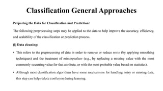
SlideShare a Scribd company logo
1 of 54
DATA WAREHOUSING AND
DATA MINING
UNIT – 3
Prepared by
Mr. P. Nandakumar
Assistant Professor,
Department of IT, SVCET
UNIT-III
Classification and Prediction: Issues Regarding Classification and
Prediction – Classification by Decision Tree Introduction – Bayesian
Classification – Rule Based Classification – Classification by Back
propagation – Support Vector Machines – Associative Classification
– Lazy Learners – Other Classification Methods – Prediction –
Accuracy and Error Measures – Evaluating the Accuracy of a
Classifier or Predictor – Ensemble Methods – Model Section.
Classification and Prediction
• Classification and prediction are two forms of data analysis that can be used to extract models
describing important data classes or to predict future data trends.
• Classification predicts categorical (discrete, unordered) labels, prediction models continuous valued
functions.
• For example, we can build a classification model to categorize bank loan applications as either safe
or risky, or a prediction model to predict the expenditures of potential customers on computer
equipment given their income and occupation.
• A predictor is constructed that predicts a continuous-valued function, or ordered value, as opposed to
a categorical label.
Classification and Prediction
• Regression analysis is a statistical methodology that is most often used for numeric prediction.
• Many classification and prediction methods have been proposed by researchers in machine learning,
pattern recognition, and statistics.
• Most algorithms are memory resident, typically assuming a small data size. Recent data mining
research has built on such work, developing scalable classification and prediction techniques capable
of handling large disk-resident data.
Classification General Approaches
Preparing the Data for Classification and Prediction:
The following preprocessing steps may be applied to the data to help improve the accuracy, efficiency,
and scalability of the classification or prediction process.
(i) Data cleaning:
• This refers to the preprocessing of data in order to remove or reduce noise (by applying smoothing
techniques) and the treatment of missingvalues (e.g., by replacing a missing value with the most
commonly occurring value for that attribute, or with the most probable value based on statistics).
• Although most classification algorithms have some mechanisms for handling noisy or missing data,
this step can help reduce confusion during learning.
Classification General Approaches
(ii) Relevance analysis:
• Many of the attributes in the data may be redundant.
• Correlation analysis can be used to identify whether any two given attributes are statistically related.
• For example, a strong correlation between attributes A1 and A2 would suggest that one of the two
could be removed from further analysis.
• A database may also contain irrelevant attributes. Attribute subset selection can be used in these
cases to find a reduced set of attributes such that the resulting probability distribution of the data
classes is as close as possible to the original distribution obtained using all attributes.
• Hence, relevance analysis, in the form of correlation analysis and attribute subset selection, can be
used to detect attributes that do not contribute to the classification or prediction task.
• Such analysis can help improve classification efficiency and scalability.
Classification General Approaches
(iii) Data Transformation And Reduction
• The data may be transformed by normalization, particularly when neural networks or methods involving
distance measurements are used in the learning step.
• Normalization involves scaling all values for a given attribute so that they fall within a small specified range,
such as -1 to +1 or 0 to 1.
• The data can also be transformed by generalizing it to higher-level concepts. Concept hierarchies may be used
for this purpose. This is particularly useful for continuous valued attributes.
• For example, numeric values for the attribute income can be generalized to discrete ranges, such as low, medium,
and high. Similarly, categorical attributes, like street, can be generalized to higher-level concepts, like city.
• Data can also be reduced by applying many other methods, ranging from wavelet transformation and principle
components analysis to discretization techniques, such as binning, histogram analysis, and clustering .
Comparing Classification and
Prediction Methods
Accuracy:
• The accuracy of a classifier refers to the ability of a given classifier to correctly predict the class label of new or
previously unseen data (i.e., tuples without class label information).
• The accuracy of a predictor refers to how well a given predictor can guess the value of the predicted attribute for
new or previously unseen data.
Speed:
• This refers to the computational costs involved in generating and using the given classifier or predictor.
Robustness:
• This is the ability of the classifier or predictor to make correct predictions given noisy data or data with missing
values.
Scalability:
• This refers to the ability to construct the classifier or predictor efficiently given large amounts of data.
Interpretability:
• This refers to the level of understanding and insight that is providedby the classifier or predictor.
• Interpretability is subjective and therefore more difficult to assess.
Decision Tree Algorithm
• Decision tree induction is the learning of decision trees from class-labeled training tuples.
• A decision tree is a flowchart-like tree structure, where
Each internal node denotes a test on an attribute.
Each branch represents an outcome of the test.
Each leaf node holds a class label.
The topmost node in a tree is the root node.
• The construction of decision tree classifiers does not
require any domain knowledge or parameter setting,
and therefore I appropriate for exploratory knowledge
discovery.
• Decision trees can handle high dimensional data.
• Their representation of acquired knowledge in tree
form is intuitive and generally easy to assimilate by humans.
• The learning and classification steps of decision tree induction are simple and fast. In general, decision tree
classifiers have good accuracy.
• Decision tree induction algorithms have been used for classification in many application areas, such as
medicine, manufacturing and production, financial analysis, astronomy, and molecular biology.
Algorithm For Decision Tree Induction
• The algorithm is called with three parameters:
➢ Data partition
➢ Attribute list
➢ Attribute selection method
• The parameter attribute list is a list of attributes describing the tuples.
• Attribute selection method specifies a heuristic procedure for selecting the attribute that
• ―best discriminates the given tuples according to class.
• The tree starts as a single node, N, representing the training tuples in D.
• If the tuples in D are all of the same class, then node N becomes a leaf and is labeled with that class .
• All of the terminating conditions are explained at the end of the algorithm. Otherwise, the algorithm calls
Attribute selection method to determine the splitting criterion.
• The splitting criterion tells us which attribute to test at node N by determining the ―best way to separate or
partition the tuples in D into individual classes.
Bayesian Classification
 Bayesian classifiers are statistical classifiers.
 They can predict class membership probabilities, such as the probability that a given tuple belongs to a
particular class.
 Bayesian classification is based on Bayes’ theorem.
Bayes’ Theorem:
• Let X be a data tuple. In Bayesian terms, X is considered ―evidence and it is described by measurements made
on a set of n attributes.
• Let H be some hypothesis, such as that the data tuple X belongs to a specified class C.
• For classification problems, we want to determine P(H|X), the probability that the hypothesis H holds given the
―evidence‖ or observed data tuple X.
• P(H|X) is the posterior probability, or a posteriori probability, of H conditioned on X. Bayes’ theorem is useful
in that it provides a way of calculating the posterior probability, P(H|X), from P(H), P(X|H), and P(X).
Naïve Bayesian Classifier
The naïve Bayesian classifier, or simple Bayesian classifier, works as follows:
1. Let D be a training set of tuples and their associated class labels. As usual, each tuple is represented
by an n-dimensional attribute vector, X = (x1, x2, …,xn), depicting n measurements made on the tuple
from n attributes, respectively, A1, A2, …, An.
2. Suppose that there are m classes, C1, C2, …, Cm. Given a tuple, X, the classifier will predict that X
belongs to the class having the highest posterior probability, conditioned on X.
• That is, the naïve Bayesian classifier predicts that tuple X belongs to the class Ci if and only if
• Thus we maximize P(CijX). The class Ci for which P(CijX) is maximized is called the maximum
posteriori hypothesis. By Bayes’ theorem
Naïve Bayesian Classifier
3. As P(X) is constant for all classes, only P(X|Ci)P(Ci) need be maximized. If the class prior
probabilities are not known, then it is commonly assumed that the classes are equally likely, that is,
P(C1) = P(C2) = …= P(Cm), and we would therefore maximize P(X|Ci). Otherwise, we maximize
P(X|Ci)P(Ci).
4. Given data sets with many attributes, it would be extremely computationally expensive to compute
P(X|Ci). In order to reduce computation in evaluating P(X|Ci), the naive assumption of class
conditional independence is made. This presumes that the values of the attributes are conditionally
independent of one another, given the class label of the tuple. Thus,
We can easily estimate the probabilities P(x1|Ci), P(x2|Ci), : : : , P(xn|Ci) from the training tuples. For
each attribute, we look at whether the attribute is categorical or continuous- valued. For instance, to
compute P(X|Ci), we consider the following:
Naïve Bayesian Classifier
• If Ak is categorical, then P(xk|Ci) is the number of tuples of class Ci in D having the value xkfor Ak,
divided by |Ci,D| the number of tuples of class Ciin D.
• If Ak is continuous-valued, then we need to do a bit more work, but the calculation is pretty
straightforward.
• A continuous-valued attribute is typically assumed to have a Gaussian distribution with a mean μ and
standard deviation , defined by
5. In order to predict the class label of X, P(XjCi)P(Ci) is evaluated for each class Ci. The classifier
predicts that the class label of tuple X is the class Ci if and only if
Rule Based Classification
• Rule-based classification in data mining is a technique in which class decisions are taken based on
various “if...then… else” rules. Thus, we define it as a classification type governed by a set of IF-
THEN rules. We write an IF-THEN rule as:
“IF condition THEN conclusion.”
IF-THEN Rule
To define the IF-THEN rule, we can split it into two parts:
• Rule Antecedent: This is the “if condition” part of the rule. This part is present in the LHS(Left
Hand Side). The antecedent can have one or more attributes as conditions, with logic AND operator.
• Rule Consequent: This is present in the rule's RHS(Right Hand Side). The rule consequent consists
of the class prediction.
Rule Based Classification
Assessment of Rule
In rule-based classification in data mining, there are two factors based on which we can access the
rules. These are:
Coverage of Rule: The fraction of the records which satisfy the antecedent conditions of a particular
rule is called the coverage of that rule.
We can calculate this by dividing the number of records satisfying the rule(n1) by the total number of
records(n).
Coverage(R) = n1/n
Accuracy of a rule: The fraction of the records that satisfy the antecedent conditions and meet the
consequent values of a rule is called the accuracy of that rule.
We can calculate this by dividing the number of records satisfying the consequent values(n2) by the
number of records satisfying the rule(n1).
Accuracy(R) = n2/n1
Rule Based Classification
Properties of Rule-Based Classifiers
There are two significant properties of rule-based classification in data mining. They are:
1. Rules may not be mutually exclusive
2. Rules may not be exhaustive
Implementation of Rule-Based Classifier
We have two different kinds of methods for implementing rule-based classification in data mining.
They are:
1. Direct Method - 1R Algorithm and Sequential Covering Algorithm
2. Indirect Method - In the indirect method of rule-based classification in data mining, we extract
rules from different other classification models. Some prominent classifications from which we
extract the rules are decision trees and neural networks.
Advantages of Rule Based Classification
The rule-based classification is easy to generate.
It is highly expressive in nature and very easy to understand.
It assists in the classification of new records in significantly less time and very quickly.
It helps us to handle redundant values during classification properly.
The performance of the rule-based classification is comparable to that of a decision tree.
Backpropagation in Data Mining
Backpropagation is an algorithm that backpropagates the errors from the output nodes to the input
nodes.
Therefore, it is simply referred to as the backward propagation of errors.
It uses in the vast applications of neural networks in data mining like Character recognition,
Signature verification, etc.
Backpropagation is a widely used algorithm for training feedforward neural networks.
It computes the gradient of the loss function with respect to the network weights. It is very efficient,
rather than naively directly computing the gradient concerning each weight.
This efficiency makes it possible to use gradient methods to train multi-layer networks and update
weights to minimize loss; variants such as gradient descent or stochastic gradient descent are often
used.
The backpropagation algorithm works by computing the gradient of the loss function with respect to
each weight via the chain rule, computing the gradient layer by layer, and iterating backward from
the last layer to avoid redundant computation of intermediate terms in the chain rule.
Backpropagation in Data Mining
Features and Working of
Backpropagation
Features:
it is the gradient descent method as used in the case of simple perceptron network with the
differentiable unit.
it is different from other networks in respect to the process by which the weights are calculated
during the learning period of the network.
training is done in the three stages :
the feed-forward of input training pattern
the calculation and backpropagation of the error
updation of the weight
Working:
Neural networks use supervised learning to generate output vectors from input vectors that the
network operates on.
It Compares generated output to the desired output and generates an error report if the result does not
match the generated output vector.
Then it adjusts the weights according to the bug report to get your desired output.
Backpropagation Algorithm
Step 1: Inputs X, arrive through the preconnected path.
Step 2: The input is modeled using true weights W. Weights are usually chosen randomly.
Step 3: Calculate the output of each neuron from the input layer to the hidden layer to the output layer.
Step 4: Calculate the error in the outputs
Backpropagation Error= Actual Output – Desired Output
Step 5: From the output layer, go back to the hidden layer to adjust the weights to reduce the error.
Step 6: Repeat the process until the desired output is achieved.
Backpropagation Algorithm
Parameters :
• x = inputs training vector x=(x1,x2,…………xn).
• t = target vector t=(t1,t2……………tn).
• δk = error at output unit.
• δj = error at hidden layer.
• α = learning rate.
• V0j = bias of hidden unit j.
Backpropagation Training Algorithm
Step 1: Initialize weight to small random values.
Step 2: While the steps stopping condition is to be false do step 3 to 10.
Step 3: For each training pair do step 4 to 9 (Feed-Forward).
Step 4: Each input unit receives the signal unit and transmits the signal xi signal to all the units.
Step 5 : Each hidden unit Zj (z=1 to a) sums its weighted input signal to calculate its net input
zinj = v0j + Σxivij ( i=1 to n)
Applying activation function zj = f(zinj) and sends this signals to all units in the layer about i.e
output units
For each output l=unit yk = (k=1 to m) sums its weighted input signals.
yink = w0k + Σ ziwjk (j=1 to a)
and applies its activation function to calculate the output signals.
yk = f(yink)
Backpropagation Training Algorithm -
Backpropagation Error
Step 6: Each output unit yk (k=1 to n) receives a target pattern corresponding to an input pattern then
error is calculated as:
δk = ( tk – yk ) + yink
Step 7: Each hidden unit Zj (j=1 to a) sums its input from all units in the layer above
δinj = Σ δj wjk
The error information term is calculated as :
δj = δinj + zinj
Backpropagation Training Algorithm -
Updation of weight and bias
Step 8: Each output unit yk (k=1 to m) updates its bias and weight (j=1 to a). The weight correction term
is given by :
Δ wjk = α δk zj
and the bias correction term is given by Δwk = α δk.
therefore wjk(new) = wjk(old) + Δ wjk
w0k(new) = wok(old) + Δ wok
for each hidden unit zj (j=1 to a) update its bias and weights (i=0 to n) the weight connection
term
Δ vij = α δj xi
and the bias connection on term
Δ v0j = α δj
Therefore vij(new) = vij(old) + Δvij
v0j(new) = v0j(old) + Δv0j
Step 9: Test the stopping condition. The stopping condition can be the minimization of error, number of
epochs.
Need for Backpropagation and Types
Need:
Backpropagation is “backpropagation of errors” and is very useful for training neural networks. It’s fast,
easy to implement, and simple. Backpropagation does not require any parameters to be set, except the
number of inputs. Backpropagation is a flexible method because no prior knowledge of the network is
required.
Types of Backpropagation
There are two types of backpropagation networks.
Static backpropagation: Static backpropagation is a network designed to map static inputs for static
outputs. These types of networks are capable of solving static classification problems such as OCR
(Optical Character Recognition).
Recurrent backpropagation: Recursive backpropagation is another network used for fixed-point
learning. Activation in recurrent backpropagation is feed-forward until a fixed value is reached. Static
backpropagation provides an instant mapping, while recurrent backpropagation does not provide an
instant mapping
Advantages and Disadvantages of
Backpropagation
It is simple, fast, and easy to program.
Only numbers of the input are tuned, not any other parameter.
It is flexible and efficient.
No need for users to learn any special functions.
• It is sensitive to noisy data and irregularities. Noisy data can lead to inaccurate results.
• Performance is highly dependent on input data.
• Spending too much time training.
• The matrix-based approach is preferred over a mini-batch.
Support Vector Machine
Support Vector Machine or SVM is one of the most popular Supervised Learning algorithms, which is
used for Classification as well as Regression problems. However, primarily, it is used for Classification
problems in Machine Learning.
The goal of the SVM algorithm is to create the best line or decision boundary that can segregate n-
dimensional space into classes so that we can easily put the new data point in the correct category in the
future. This best decision boundary is called a hyperplane.
SVM chooses the extreme points/vectors that help in creating the hyperplane. These extreme cases are
called as support vectors, and hence algorithm is termed as Support Vector Machine.
Support Vector Machine
SVM algorithm can be used for Face detection, image classification, text categorization, etc.
Support Vector Machine
Types of SVM
Linear SVM: Linear SVM is used for linearly separable data, which means if a dataset can be classified
into two classes by using a single straight line, then such data is termed as linearly separable data, and
classifier is used called as Linear SVM classifier.
Non-linear SVM: Non-Linear SVM is used for non-linearly separated data, which means if a dataset
cannot be classified by using a straight line, then such data is termed as non-linear data and classifier used
is called as Non-linear SVM classifier.
Support Vector Machine
Advantages of SVM
Effective in high-dimensional cases.
Its memory is efficient as it uses a subset of training points in the decision function called support
vectors.
Different kernel functions can be specified for the decision functions and its possible to specify custom
kernels.
Support Vector Machine
Hyperplane and Support Vectors in the SVM algorithm:
Hyperplane: There can be multiple lines/decision boundaries to segregate the classes in n-dimensional
space, but we need to find out the best decision boundary that helps to classify the data points. This best
boundary is known as the hyperplane of SVM.
The dimensions of the hyperplane depend on the features present in the dataset, which means if there are 2
features (as shown in image), then hyperplane will be a straight line. And if there are 3 features, then
hyperplane will be a 2-dimension plane.
We always create a hyperplane that has a maximum margin, which means the maximum distance between
the data points.
Support Vector Machine
Support Vectors:
The data points or vectors that are the closest to the hyperplane and which affect the position of the
hyperplane are termed as Support Vector. Since these vectors support the hyperplane, hence called a
Support vector.
Associative Classification
Associative classification is a common classification learning method in data mining, which applies
association rule detection methods and classification to create classification models.
Bing Liu Et Al was the first to propose associative classification, in which he defined a model whose rule
is “the right-hand side is constrained to be the attribute of the classification class”.
An associative classifier is a supervised learning model that uses association rules to assign a target value.
The model generated by the association classifier and used to label new records consists of association
rules that produce class labels.
Therefore, they can also be thought of as a list of “if-then” clauses: if a record meets certain criteria
(specified on the left side of the rule, also known as antecedents), it is marked (or scored) according to
the rule’s category on the right.
Types of Associative Classification
1. CBA (Classification Based on Associations): It uses association rule techniques to classify data,
which proves to be more accurate than traditional classification techniques. It has to face the sensitivity of
the minimum support threshold. When a lower minimum support threshold is specified, a large number of
rules are generated.
2. CMAR (Classification based on Multiple Association Rules): It uses an efficient FP-tree, which
consumes less memory and space compared to Classification Based on Associations. The FP-tree will not
always fit in the main memory, especially when the number of attributes is large.
3. CPAR (Classification based on Predictive Association Rules): Classification based on predictive
association rules combines the advantages of association classification and traditional rule-based
classification. Classification based on predictive association rules uses a greedy algorithm to generate
rules directly from training data. Furthermore, classification based on predictive association rules
generates and tests more rules than traditional rule-based classifiers to avoid missing important rules.
Lazy Learners
Lazy Learners
As the name suggests, such kind of learners waits for the testing data to be appeared after storing the
training data. Classification is done only after getting the testing data. They spend less time on training but
more time on predicting. Examples of lazy learners are K-nearest neighbor and case-based reasoning.
Eager Learners
As opposite to lazy learners, eager learners construct classification model without waiting for the testing
data to be appeared after storing the training data. They spend more time on training but less time on
predicting. Examples of eager learners are Decision Trees, Naïve Bayes and Artificial Neural Networks
(ANN).
Other Classification Methods
Genetic Algorithms:
Genetic Algorithm: based on an analogy to biological evolution
Rough Set Approach:
Rough sets are used to approximately or ―roughly define equivalent classes
Fuzzy Set approaches:
 Fuzzy logic uses truth values between 0.0 and 1.0 to represent the degree of membership (such as using
fuzzy membership graph)
 Attribute values are converted to fuzzy values
Prediction, Accuracy and Error Measures
The predictive accuracy describes whether the predicted values match the actual values of the target field
within the incertitude due to statistical fluctuations and noise in the input data values.
Accuracy is one metric for evaluating classification models. Informally, accuracy is the fraction of
predictions our model got right. Formally, accuracy has the following definition:
Accuracy = Number of correct predictions / Total number of predictions
For binary classification, accuracy can also be calculated in terms of positives and negatives as follows:
Accuracy = TP+TN / TP+TN+FP+FN
Where TP = True Positives, TN = True Negatives, FP = False Positives, and FN = False Negatives.
Error Measures: It refers to any problem resulting from the measurement process. In other words, the
recorded data values differ from true values to some extent. The difference between measured and true
value is called the error.
Evaluate Accuracy of Classifier in Data
Mining
HoldOut
In the holdout method, the largest dataset is randomly divided into three subsets:
1. A training set is a subset of the dataset which are been used to build predictive models.
2. The validation set is a subset of the dataset which is been used to assess the performance of the model
built in the training phase.
3. Test sets or unseen examples are the subset of the dataset to assess the likely future performance of
the model.
Evaluate Accuracy of Classifier in Data
Mining
Evaluate Accuracy of Classifier in Data
Mining
Random Subsampling
Random subsampling is a variation of the holdout method. The holdout method is been repeated K
times.
The holdout subsampling involves randomly splitting the data into a training set and a test set.
On the training set the data is been trained and the mean square error (MSE) is been obtained from the
predictions on the test set.
As MSE is dependent on the split, this method is not recommended. So a new split can give you a new
MSE.
Evaluate Accuracy of Classifier in Data
Mining
Cross-Validation
K-fold cross-validation is been used when there is only a limited amount of data available, to achieve an
unbiased estimation of the performance of the model.
Here, we divide the data into K subsets of equal sizes.
We build models K times, each time leaving out one of the subsets from the training, and use it as the
test set.
If K equals the sample size, then this is called a “Leave-One-Out”.
Evaluate Accuracy of Classifier in Data
Mining
Bootstrapping
Bootstrapping is one of the techniques which is used to make the estimations from the data by taking an
average of the estimates from smaller data samples.
The bootstrapping method involves the iterative resampling of a dataset with replacement.
On resampling instead of only estimating the statistics once on complete data, we can do it many times.
Repeating this multiple times helps to obtain a vector of estimates.
Bootstrapping can compute variance, expected value, and other relevant statistics of these estimates.
Ensemble Methods
Ensemble learning helps improve machine learning results by combining several models. This approach
allows the production of better predictive performance compared to a single model.
Advantage : Improvement in predictive accuracy.
Disadvantage : It is difficult to understand an ensemble of classifiers.
Ensemble Methods
Dietterich(2002) showed that ensembles overcome three problems –
Statistical Problem – The Statistical Problem arises when the hypothesis space is too large for the amount
of available data. Hence, there are many hypotheses with the same accuracy on the data and the learning
algorithm chooses only one of them! There is a risk that the accuracy of the chosen hypothesis is low on
unseen data!
Computational Problem – The Computational Problem arises when the learning algorithm cannot
guarantees finding the best hypothesis.
Representational Problem – The Representational Problem arises when the hypothesis space does not
contain any good approximation of the target class(es).
Types of Ensemble Methods
Bagging Ensemble Learning
Bootstrap aggregation, or bagging for short, is an ensemble learning method that seeks a diverse group of
ensemble members by varying the training data.
Stacking Ensemble Learning
Stacked Generalization, or stacking for short, is an ensemble method that seeks a diverse group of
members by varying the model types fit on the training data and using a model to combine predictions.
Boosting Ensemble Learning
Boosting is an ensemble method that seeks to change the training data to focus attention on examples that
previous fit models on the training dataset have gotten wrong.
Types of Ensemble Methods
Voting and Averaging Based Ensemble Methods
Voting and averaging are two of the easiest examples of ensemble learning in machine learning. They are
both easy to understand and implement. Voting is used for classification and averaging is used for
regression.
Sample Architecture of Ensemble Methods
Model Selection
Model Selection is the process of choosing the best model among all the potential candidate models for a
given problem.
The aim of the model selection process is to select a machine learning algorithm that evaluates to perform
well against all the different parameters.
It is as essential as any other technique for the model performance improvement, such as data pre-
processing that involves cleaning, transforming, and scaling the data before training, feature engineering
to transform features and create new ones, hyperparameter tuning to find the best combination of
parameters to optimize the model performance and many more.
Model Selection
• Akaike
Information
Criterion (AIC
Model
Selection)
• Bayesian
Information
Criterion (BIC
Model
Selection)
• Bayesian
Model
Averaging
(BMA Model
Selection)

More Related Content

Similar to UNIT 3: Data Warehousing and Data Mining

A Decision Tree Based Classifier for Classification & Prediction of Diseases
A Decision Tree Based Classifier for Classification & Prediction of DiseasesA Decision Tree Based Classifier for Classification & Prediction of Diseases
A Decision Tree Based Classifier for Classification & Prediction of Diseasesijsrd.com
 
Chapter 11 Data Analysis Classification and Tabulation
Chapter 11 Data Analysis Classification and TabulationChapter 11 Data Analysis Classification and Tabulation
Chapter 11 Data Analysis Classification and TabulationInternational advisers
 
IRJET- Study and Evaluation of Classification Algorithms in Data Mining
IRJET- Study and Evaluation of Classification Algorithms in Data MiningIRJET- Study and Evaluation of Classification Algorithms in Data Mining
IRJET- Study and Evaluation of Classification Algorithms in Data MiningIRJET Journal
 
5. Machine Learning.pptx
5.  Machine Learning.pptx5.  Machine Learning.pptx
5. Machine Learning.pptxssuser6654de1
 
Sampling and Data_Update.ppt
Sampling and Data_Update.pptSampling and Data_Update.ppt
Sampling and Data_Update.pptMdShohelRana69
 
Introduction to Data Analysis for Nurse Researchers
Introduction to Data Analysis for Nurse ResearchersIntroduction to Data Analysis for Nurse Researchers
Introduction to Data Analysis for Nurse ResearchersRupa Verma
 
Predictive analytics
Predictive analyticsPredictive analytics
Predictive analyticsDinakar nk
 
Big Data Analytics - Unit 3.pptx
Big Data Analytics - Unit 3.pptxBig Data Analytics - Unit 3.pptx
Big Data Analytics - Unit 3.pptxPlacementsBCA
 
Biostatistics mean median mode unit 1.pptx
Biostatistics mean median mode unit 1.pptxBiostatistics mean median mode unit 1.pptx
Biostatistics mean median mode unit 1.pptxSailajaReddyGunnam
 
Data mining approaches and methods
Data mining approaches and methodsData mining approaches and methods
Data mining approaches and methodssonangrai
 
CS 402 DATAMINING AND WAREHOUSING -MODULE 3
CS 402 DATAMINING AND WAREHOUSING -MODULE 3CS 402 DATAMINING AND WAREHOUSING -MODULE 3
CS 402 DATAMINING AND WAREHOUSING -MODULE 3NIMMYRAJU
 
20IT501_DWDM_PPT_Unit_IV.ppt
20IT501_DWDM_PPT_Unit_IV.ppt20IT501_DWDM_PPT_Unit_IV.ppt
20IT501_DWDM_PPT_Unit_IV.pptSamPrem3
 
20IT501_DWDM_PPT_Unit_IV.ppt
20IT501_DWDM_PPT_Unit_IV.ppt20IT501_DWDM_PPT_Unit_IV.ppt
20IT501_DWDM_PPT_Unit_IV.pptPalaniKumarR2
 
Data Mining StepsProblem Definition Market AnalysisC
Data Mining StepsProblem Definition Market AnalysisCData Mining StepsProblem Definition Market AnalysisC
Data Mining StepsProblem Definition Market AnalysisCsharondabriggs
 
classification in data mining and data warehousing.pdf
classification in data mining and data warehousing.pdfclassification in data mining and data warehousing.pdf
classification in data mining and data warehousing.pdf321106410027
 
Unit 3 – AIML.pptx
Unit 3 – AIML.pptxUnit 3 – AIML.pptx
Unit 3 – AIML.pptxhiblooms
 

Similar to UNIT 3: Data Warehousing and Data Mining (20)

A Decision Tree Based Classifier for Classification & Prediction of Diseases
A Decision Tree Based Classifier for Classification & Prediction of DiseasesA Decision Tree Based Classifier for Classification & Prediction of Diseases
A Decision Tree Based Classifier for Classification & Prediction of Diseases
 
Chapter 11 Data Analysis Classification and Tabulation
Chapter 11 Data Analysis Classification and TabulationChapter 11 Data Analysis Classification and Tabulation
Chapter 11 Data Analysis Classification and Tabulation
 
IRJET- Study and Evaluation of Classification Algorithms in Data Mining
IRJET- Study and Evaluation of Classification Algorithms in Data MiningIRJET- Study and Evaluation of Classification Algorithms in Data Mining
IRJET- Study and Evaluation of Classification Algorithms in Data Mining
 
5. Machine Learning.pptx
5.  Machine Learning.pptx5.  Machine Learning.pptx
5. Machine Learning.pptx
 
Sampling and Data_Update.ppt
Sampling and Data_Update.pptSampling and Data_Update.ppt
Sampling and Data_Update.ppt
 
Introduction to Data Analysis for Nurse Researchers
Introduction to Data Analysis for Nurse ResearchersIntroduction to Data Analysis for Nurse Researchers
Introduction to Data Analysis for Nurse Researchers
 
Predictive analytics
Predictive analyticsPredictive analytics
Predictive analytics
 
Data discretization
Data discretizationData discretization
Data discretization
 
Big Data Analytics - Unit 3.pptx
Big Data Analytics - Unit 3.pptxBig Data Analytics - Unit 3.pptx
Big Data Analytics - Unit 3.pptx
 
Biostatistics mean median mode unit 1.pptx
Biostatistics mean median mode unit 1.pptxBiostatistics mean median mode unit 1.pptx
Biostatistics mean median mode unit 1.pptx
 
Datamining
DataminingDatamining
Datamining
 
Data mining approaches and methods
Data mining approaches and methodsData mining approaches and methods
Data mining approaches and methods
 
CS 402 DATAMINING AND WAREHOUSING -MODULE 3
CS 402 DATAMINING AND WAREHOUSING -MODULE 3CS 402 DATAMINING AND WAREHOUSING -MODULE 3
CS 402 DATAMINING AND WAREHOUSING -MODULE 3
 
classification.pptx
classification.pptxclassification.pptx
classification.pptx
 
20IT501_DWDM_PPT_Unit_IV.ppt
20IT501_DWDM_PPT_Unit_IV.ppt20IT501_DWDM_PPT_Unit_IV.ppt
20IT501_DWDM_PPT_Unit_IV.ppt
 
20IT501_DWDM_PPT_Unit_IV.ppt
20IT501_DWDM_PPT_Unit_IV.ppt20IT501_DWDM_PPT_Unit_IV.ppt
20IT501_DWDM_PPT_Unit_IV.ppt
 
Data Mining StepsProblem Definition Market AnalysisC
Data Mining StepsProblem Definition Market AnalysisCData Mining StepsProblem Definition Market AnalysisC
Data Mining StepsProblem Definition Market AnalysisC
 
classification in data mining and data warehousing.pdf
classification in data mining and data warehousing.pdfclassification in data mining and data warehousing.pdf
classification in data mining and data warehousing.pdf
 
18 ijcse-01232
18 ijcse-0123218 ijcse-01232
18 ijcse-01232
 
Unit 3 – AIML.pptx
Unit 3 – AIML.pptxUnit 3 – AIML.pptx
Unit 3 – AIML.pptx
 

More from Nandakumar P

UNIT - 5: Data Warehousing and Data Mining
UNIT - 5: Data Warehousing and Data MiningUNIT - 5: Data Warehousing and Data Mining
UNIT - 5: Data Warehousing and Data MiningNandakumar P
 
UNIT - 4: Data Warehousing and Data Mining
UNIT - 4: Data Warehousing and Data MiningUNIT - 4: Data Warehousing and Data Mining
UNIT - 4: Data Warehousing and Data MiningNandakumar P
 
UNIT 2: Part 2: Data Warehousing and Data Mining
UNIT 2: Part 2: Data Warehousing and Data MiningUNIT 2: Part 2: Data Warehousing and Data Mining
UNIT 2: Part 2: Data Warehousing and Data MiningNandakumar P
 
UNIT 2: Part 1: Data Warehousing and Data Mining
UNIT 2: Part 1: Data Warehousing and Data MiningUNIT 2: Part 1: Data Warehousing and Data Mining
UNIT 2: Part 1: Data Warehousing and Data MiningNandakumar P
 
UNIT - 1 Part 2: Data Warehousing and Data Mining
UNIT - 1 Part 2: Data Warehousing and Data MiningUNIT - 1 Part 2: Data Warehousing and Data Mining
UNIT - 1 Part 2: Data Warehousing and Data MiningNandakumar P
 
UNIT - 1 : Part 1: Data Warehousing and Data Mining
UNIT - 1 : Part 1: Data Warehousing and Data MiningUNIT - 1 : Part 1: Data Warehousing and Data Mining
UNIT - 1 : Part 1: Data Warehousing and Data MiningNandakumar P
 
UNIT - 5 : 20ACS04 – PROBLEM SOLVING AND PROGRAMMING USING PYTHON
UNIT - 5 : 20ACS04 – PROBLEM SOLVING AND PROGRAMMING USING PYTHONUNIT - 5 : 20ACS04 – PROBLEM SOLVING AND PROGRAMMING USING PYTHON
UNIT - 5 : 20ACS04 – PROBLEM SOLVING AND PROGRAMMING USING PYTHONNandakumar P
 
UNIT - 2 : 20ACS04 – PROBLEM SOLVING AND PROGRAMMING USING PYTHON
UNIT - 2 : 20ACS04 – PROBLEM SOLVING AND PROGRAMMING USING PYTHONUNIT - 2 : 20ACS04 – PROBLEM SOLVING AND PROGRAMMING USING PYTHON
UNIT - 2 : 20ACS04 – PROBLEM SOLVING AND PROGRAMMING USING PYTHONNandakumar P
 
UNIT-1 : 20ACS04 – PROBLEM SOLVING AND PROGRAMMING USING PYTHON
UNIT-1 : 20ACS04 – PROBLEM SOLVING AND PROGRAMMING USING PYTHON UNIT-1 : 20ACS04 – PROBLEM SOLVING AND PROGRAMMING USING PYTHON
UNIT-1 : 20ACS04 – PROBLEM SOLVING AND PROGRAMMING USING PYTHON Nandakumar P
 
Python Course for Beginners
Python Course for BeginnersPython Course for Beginners
Python Course for BeginnersNandakumar P
 
CS6601-Unit 4 Distributed Systems
CS6601-Unit 4 Distributed SystemsCS6601-Unit 4 Distributed Systems
CS6601-Unit 4 Distributed SystemsNandakumar P
 
Unit-4 Professional Ethics in Engineering
Unit-4 Professional Ethics in EngineeringUnit-4 Professional Ethics in Engineering
Unit-4 Professional Ethics in EngineeringNandakumar P
 
Unit-3 Professional Ethics in Engineering
Unit-3 Professional Ethics in EngineeringUnit-3 Professional Ethics in Engineering
Unit-3 Professional Ethics in EngineeringNandakumar P
 
Naming in Distributed Systems
Naming in Distributed SystemsNaming in Distributed Systems
Naming in Distributed SystemsNandakumar P
 
Unit 3.1 cs6601 Distributed File System
Unit 3.1 cs6601 Distributed File SystemUnit 3.1 cs6601 Distributed File System
Unit 3.1 cs6601 Distributed File SystemNandakumar P
 
Unit 3 cs6601 Distributed Systems
Unit 3 cs6601 Distributed SystemsUnit 3 cs6601 Distributed Systems
Unit 3 cs6601 Distributed SystemsNandakumar P
 
Professional Ethics in Engineering
Professional Ethics in EngineeringProfessional Ethics in Engineering
Professional Ethics in EngineeringNandakumar P
 

More from Nandakumar P (17)

UNIT - 5: Data Warehousing and Data Mining
UNIT - 5: Data Warehousing and Data MiningUNIT - 5: Data Warehousing and Data Mining
UNIT - 5: Data Warehousing and Data Mining
 
UNIT - 4: Data Warehousing and Data Mining
UNIT - 4: Data Warehousing and Data MiningUNIT - 4: Data Warehousing and Data Mining
UNIT - 4: Data Warehousing and Data Mining
 
UNIT 2: Part 2: Data Warehousing and Data Mining
UNIT 2: Part 2: Data Warehousing and Data MiningUNIT 2: Part 2: Data Warehousing and Data Mining
UNIT 2: Part 2: Data Warehousing and Data Mining
 
UNIT 2: Part 1: Data Warehousing and Data Mining
UNIT 2: Part 1: Data Warehousing and Data MiningUNIT 2: Part 1: Data Warehousing and Data Mining
UNIT 2: Part 1: Data Warehousing and Data Mining
 
UNIT - 1 Part 2: Data Warehousing and Data Mining
UNIT - 1 Part 2: Data Warehousing and Data MiningUNIT - 1 Part 2: Data Warehousing and Data Mining
UNIT - 1 Part 2: Data Warehousing and Data Mining
 
UNIT - 1 : Part 1: Data Warehousing and Data Mining
UNIT - 1 : Part 1: Data Warehousing and Data MiningUNIT - 1 : Part 1: Data Warehousing and Data Mining
UNIT - 1 : Part 1: Data Warehousing and Data Mining
 
UNIT - 5 : 20ACS04 – PROBLEM SOLVING AND PROGRAMMING USING PYTHON
UNIT - 5 : 20ACS04 – PROBLEM SOLVING AND PROGRAMMING USING PYTHONUNIT - 5 : 20ACS04 – PROBLEM SOLVING AND PROGRAMMING USING PYTHON
UNIT - 5 : 20ACS04 – PROBLEM SOLVING AND PROGRAMMING USING PYTHON
 
UNIT - 2 : 20ACS04 – PROBLEM SOLVING AND PROGRAMMING USING PYTHON
UNIT - 2 : 20ACS04 – PROBLEM SOLVING AND PROGRAMMING USING PYTHONUNIT - 2 : 20ACS04 – PROBLEM SOLVING AND PROGRAMMING USING PYTHON
UNIT - 2 : 20ACS04 – PROBLEM SOLVING AND PROGRAMMING USING PYTHON
 
UNIT-1 : 20ACS04 – PROBLEM SOLVING AND PROGRAMMING USING PYTHON
UNIT-1 : 20ACS04 – PROBLEM SOLVING AND PROGRAMMING USING PYTHON UNIT-1 : 20ACS04 – PROBLEM SOLVING AND PROGRAMMING USING PYTHON
UNIT-1 : 20ACS04 – PROBLEM SOLVING AND PROGRAMMING USING PYTHON
 
Python Course for Beginners
Python Course for BeginnersPython Course for Beginners
Python Course for Beginners
 
CS6601-Unit 4 Distributed Systems
CS6601-Unit 4 Distributed SystemsCS6601-Unit 4 Distributed Systems
CS6601-Unit 4 Distributed Systems
 
Unit-4 Professional Ethics in Engineering
Unit-4 Professional Ethics in EngineeringUnit-4 Professional Ethics in Engineering
Unit-4 Professional Ethics in Engineering
 
Unit-3 Professional Ethics in Engineering
Unit-3 Professional Ethics in EngineeringUnit-3 Professional Ethics in Engineering
Unit-3 Professional Ethics in Engineering
 
Naming in Distributed Systems
Naming in Distributed SystemsNaming in Distributed Systems
Naming in Distributed Systems
 
Unit 3.1 cs6601 Distributed File System
Unit 3.1 cs6601 Distributed File SystemUnit 3.1 cs6601 Distributed File System
Unit 3.1 cs6601 Distributed File System
 
Unit 3 cs6601 Distributed Systems
Unit 3 cs6601 Distributed SystemsUnit 3 cs6601 Distributed Systems
Unit 3 cs6601 Distributed Systems
 
Professional Ethics in Engineering
Professional Ethics in EngineeringProfessional Ethics in Engineering
Professional Ethics in Engineering
 

Recently uploaded

KSHARA STURA .pptx---KSHARA KARMA THERAPY (CAUSTIC THERAPY)————IMP.OF KSHARA ...
KSHARA STURA .pptx---KSHARA KARMA THERAPY (CAUSTIC THERAPY)————IMP.OF KSHARA ...KSHARA STURA .pptx---KSHARA KARMA THERAPY (CAUSTIC THERAPY)————IMP.OF KSHARA ...
KSHARA STURA .pptx---KSHARA KARMA THERAPY (CAUSTIC THERAPY)————IMP.OF KSHARA ...M56BOOKSTORE PRODUCT/SERVICE
 
Earth Day Presentation wow hello nice great
Earth Day Presentation wow hello nice greatEarth Day Presentation wow hello nice great
Earth Day Presentation wow hello nice greatYousafMalik24
 
“Oh GOSH! Reflecting on Hackteria's Collaborative Practices in a Global Do-It...
“Oh GOSH! Reflecting on Hackteria's Collaborative Practices in a Global Do-It...“Oh GOSH! Reflecting on Hackteria's Collaborative Practices in a Global Do-It...
“Oh GOSH! Reflecting on Hackteria's Collaborative Practices in a Global Do-It...Marc Dusseiller Dusjagr
 
ECONOMIC CONTEXT - PAPER 1 Q3: NEWSPAPERS.pptx
ECONOMIC CONTEXT - PAPER 1 Q3: NEWSPAPERS.pptxECONOMIC CONTEXT - PAPER 1 Q3: NEWSPAPERS.pptx
ECONOMIC CONTEXT - PAPER 1 Q3: NEWSPAPERS.pptxiammrhaywood
 
Incoming and Outgoing Shipments in 1 STEP Using Odoo 17
Incoming and Outgoing Shipments in 1 STEP Using Odoo 17Incoming and Outgoing Shipments in 1 STEP Using Odoo 17
Incoming and Outgoing Shipments in 1 STEP Using Odoo 17Celine George
 
CELL CYCLE Division Science 8 quarter IV.pptx
CELL CYCLE Division Science 8 quarter IV.pptxCELL CYCLE Division Science 8 quarter IV.pptx
CELL CYCLE Division Science 8 quarter IV.pptxJiesonDelaCerna
 
Proudly South Africa powerpoint Thorisha.pptx
Proudly South Africa powerpoint Thorisha.pptxProudly South Africa powerpoint Thorisha.pptx
Proudly South Africa powerpoint Thorisha.pptxthorishapillay1
 
Introduction to AI in Higher Education_draft.pptx
Introduction to AI in Higher Education_draft.pptxIntroduction to AI in Higher Education_draft.pptx
Introduction to AI in Higher Education_draft.pptxpboyjonauth
 
Meghan Sutherland In Media Res Media Component
Meghan Sutherland In Media Res Media ComponentMeghan Sutherland In Media Res Media Component
Meghan Sutherland In Media Res Media ComponentInMediaRes1
 
EPANDING THE CONTENT OF AN OUTLINE using notes.pptx
EPANDING THE CONTENT OF AN OUTLINE using notes.pptxEPANDING THE CONTENT OF AN OUTLINE using notes.pptx
EPANDING THE CONTENT OF AN OUTLINE using notes.pptxRaymartEstabillo3
 
Presiding Officer Training module 2024 lok sabha elections
Presiding Officer Training module 2024 lok sabha electionsPresiding Officer Training module 2024 lok sabha elections
Presiding Officer Training module 2024 lok sabha electionsanshu789521
 
Crayon Activity Handout For the Crayon A
Crayon Activity Handout For the Crayon ACrayon Activity Handout For the Crayon A
Crayon Activity Handout For the Crayon AUnboundStockton
 
Software Engineering Methodologies (overview)
Software Engineering Methodologies (overview)Software Engineering Methodologies (overview)
Software Engineering Methodologies (overview)eniolaolutunde
 
Introduction to ArtificiaI Intelligence in Higher Education
Introduction to ArtificiaI Intelligence in Higher EducationIntroduction to ArtificiaI Intelligence in Higher Education
Introduction to ArtificiaI Intelligence in Higher Educationpboyjonauth
 
Alper Gobel In Media Res Media Component
Alper Gobel In Media Res Media ComponentAlper Gobel In Media Res Media Component
Alper Gobel In Media Res Media ComponentInMediaRes1
 
call girls in Kamla Market (DELHI) 🔝 >༒9953330565🔝 genuine Escort Service 🔝✔️✔️
call girls in Kamla Market (DELHI) 🔝 >༒9953330565🔝 genuine Escort Service 🔝✔️✔️call girls in Kamla Market (DELHI) 🔝 >༒9953330565🔝 genuine Escort Service 🔝✔️✔️
call girls in Kamla Market (DELHI) 🔝 >༒9953330565🔝 genuine Escort Service 🔝✔️✔️9953056974 Low Rate Call Girls In Saket, Delhi NCR
 
How to Configure Email Server in Odoo 17
How to Configure Email Server in Odoo 17How to Configure Email Server in Odoo 17
How to Configure Email Server in Odoo 17Celine George
 
Full Stack Web Development Course for Beginners
Full Stack Web Development Course  for BeginnersFull Stack Web Development Course  for Beginners
Full Stack Web Development Course for BeginnersSabitha Banu
 

Recently uploaded (20)

KSHARA STURA .pptx---KSHARA KARMA THERAPY (CAUSTIC THERAPY)————IMP.OF KSHARA ...
KSHARA STURA .pptx---KSHARA KARMA THERAPY (CAUSTIC THERAPY)————IMP.OF KSHARA ...KSHARA STURA .pptx---KSHARA KARMA THERAPY (CAUSTIC THERAPY)————IMP.OF KSHARA ...
KSHARA STURA .pptx---KSHARA KARMA THERAPY (CAUSTIC THERAPY)————IMP.OF KSHARA ...
 
Earth Day Presentation wow hello nice great
Earth Day Presentation wow hello nice greatEarth Day Presentation wow hello nice great
Earth Day Presentation wow hello nice great
 
“Oh GOSH! Reflecting on Hackteria's Collaborative Practices in a Global Do-It...
“Oh GOSH! Reflecting on Hackteria's Collaborative Practices in a Global Do-It...“Oh GOSH! Reflecting on Hackteria's Collaborative Practices in a Global Do-It...
“Oh GOSH! Reflecting on Hackteria's Collaborative Practices in a Global Do-It...
 
ECONOMIC CONTEXT - PAPER 1 Q3: NEWSPAPERS.pptx
ECONOMIC CONTEXT - PAPER 1 Q3: NEWSPAPERS.pptxECONOMIC CONTEXT - PAPER 1 Q3: NEWSPAPERS.pptx
ECONOMIC CONTEXT - PAPER 1 Q3: NEWSPAPERS.pptx
 
Incoming and Outgoing Shipments in 1 STEP Using Odoo 17
Incoming and Outgoing Shipments in 1 STEP Using Odoo 17Incoming and Outgoing Shipments in 1 STEP Using Odoo 17
Incoming and Outgoing Shipments in 1 STEP Using Odoo 17
 
9953330565 Low Rate Call Girls In Rohini Delhi NCR
9953330565 Low Rate Call Girls In Rohini  Delhi NCR9953330565 Low Rate Call Girls In Rohini  Delhi NCR
9953330565 Low Rate Call Girls In Rohini Delhi NCR
 
CELL CYCLE Division Science 8 quarter IV.pptx
CELL CYCLE Division Science 8 quarter IV.pptxCELL CYCLE Division Science 8 quarter IV.pptx
CELL CYCLE Division Science 8 quarter IV.pptx
 
Proudly South Africa powerpoint Thorisha.pptx
Proudly South Africa powerpoint Thorisha.pptxProudly South Africa powerpoint Thorisha.pptx
Proudly South Africa powerpoint Thorisha.pptx
 
Introduction to AI in Higher Education_draft.pptx
Introduction to AI in Higher Education_draft.pptxIntroduction to AI in Higher Education_draft.pptx
Introduction to AI in Higher Education_draft.pptx
 
Meghan Sutherland In Media Res Media Component
Meghan Sutherland In Media Res Media ComponentMeghan Sutherland In Media Res Media Component
Meghan Sutherland In Media Res Media Component
 
EPANDING THE CONTENT OF AN OUTLINE using notes.pptx
EPANDING THE CONTENT OF AN OUTLINE using notes.pptxEPANDING THE CONTENT OF AN OUTLINE using notes.pptx
EPANDING THE CONTENT OF AN OUTLINE using notes.pptx
 
Presiding Officer Training module 2024 lok sabha elections
Presiding Officer Training module 2024 lok sabha electionsPresiding Officer Training module 2024 lok sabha elections
Presiding Officer Training module 2024 lok sabha elections
 
Crayon Activity Handout For the Crayon A
Crayon Activity Handout For the Crayon ACrayon Activity Handout For the Crayon A
Crayon Activity Handout For the Crayon A
 
ESSENTIAL of (CS/IT/IS) class 06 (database)
ESSENTIAL of (CS/IT/IS) class 06 (database)ESSENTIAL of (CS/IT/IS) class 06 (database)
ESSENTIAL of (CS/IT/IS) class 06 (database)
 
Software Engineering Methodologies (overview)
Software Engineering Methodologies (overview)Software Engineering Methodologies (overview)
Software Engineering Methodologies (overview)
 
Introduction to ArtificiaI Intelligence in Higher Education
Introduction to ArtificiaI Intelligence in Higher EducationIntroduction to ArtificiaI Intelligence in Higher Education
Introduction to ArtificiaI Intelligence in Higher Education
 
Alper Gobel In Media Res Media Component
Alper Gobel In Media Res Media ComponentAlper Gobel In Media Res Media Component
Alper Gobel In Media Res Media Component
 
call girls in Kamla Market (DELHI) 🔝 >༒9953330565🔝 genuine Escort Service 🔝✔️✔️
call girls in Kamla Market (DELHI) 🔝 >༒9953330565🔝 genuine Escort Service 🔝✔️✔️call girls in Kamla Market (DELHI) 🔝 >༒9953330565🔝 genuine Escort Service 🔝✔️✔️
call girls in Kamla Market (DELHI) 🔝 >༒9953330565🔝 genuine Escort Service 🔝✔️✔️
 
How to Configure Email Server in Odoo 17
How to Configure Email Server in Odoo 17How to Configure Email Server in Odoo 17
How to Configure Email Server in Odoo 17
 
Full Stack Web Development Course for Beginners
Full Stack Web Development Course  for BeginnersFull Stack Web Development Course  for Beginners
Full Stack Web Development Course for Beginners
 

UNIT 3: Data Warehousing and Data Mining

  • 1. DATA WAREHOUSING AND DATA MINING UNIT – 3 Prepared by Mr. P. Nandakumar Assistant Professor, Department of IT, SVCET
  • 2. UNIT-III Classification and Prediction: Issues Regarding Classification and Prediction – Classification by Decision Tree Introduction – Bayesian Classification – Rule Based Classification – Classification by Back propagation – Support Vector Machines – Associative Classification – Lazy Learners – Other Classification Methods – Prediction – Accuracy and Error Measures – Evaluating the Accuracy of a Classifier or Predictor – Ensemble Methods – Model Section.
  • 3. Classification and Prediction • Classification and prediction are two forms of data analysis that can be used to extract models describing important data classes or to predict future data trends. • Classification predicts categorical (discrete, unordered) labels, prediction models continuous valued functions. • For example, we can build a classification model to categorize bank loan applications as either safe or risky, or a prediction model to predict the expenditures of potential customers on computer equipment given their income and occupation. • A predictor is constructed that predicts a continuous-valued function, or ordered value, as opposed to a categorical label.
  • 4. Classification and Prediction • Regression analysis is a statistical methodology that is most often used for numeric prediction. • Many classification and prediction methods have been proposed by researchers in machine learning, pattern recognition, and statistics. • Most algorithms are memory resident, typically assuming a small data size. Recent data mining research has built on such work, developing scalable classification and prediction techniques capable of handling large disk-resident data.
  • 5. Classification General Approaches Preparing the Data for Classification and Prediction: The following preprocessing steps may be applied to the data to help improve the accuracy, efficiency, and scalability of the classification or prediction process. (i) Data cleaning: • This refers to the preprocessing of data in order to remove or reduce noise (by applying smoothing techniques) and the treatment of missingvalues (e.g., by replacing a missing value with the most commonly occurring value for that attribute, or with the most probable value based on statistics). • Although most classification algorithms have some mechanisms for handling noisy or missing data, this step can help reduce confusion during learning.
  • 6. Classification General Approaches (ii) Relevance analysis: • Many of the attributes in the data may be redundant. • Correlation analysis can be used to identify whether any two given attributes are statistically related. • For example, a strong correlation between attributes A1 and A2 would suggest that one of the two could be removed from further analysis. • A database may also contain irrelevant attributes. Attribute subset selection can be used in these cases to find a reduced set of attributes such that the resulting probability distribution of the data classes is as close as possible to the original distribution obtained using all attributes. • Hence, relevance analysis, in the form of correlation analysis and attribute subset selection, can be used to detect attributes that do not contribute to the classification or prediction task. • Such analysis can help improve classification efficiency and scalability.
  • 7. Classification General Approaches (iii) Data Transformation And Reduction • The data may be transformed by normalization, particularly when neural networks or methods involving distance measurements are used in the learning step. • Normalization involves scaling all values for a given attribute so that they fall within a small specified range, such as -1 to +1 or 0 to 1. • The data can also be transformed by generalizing it to higher-level concepts. Concept hierarchies may be used for this purpose. This is particularly useful for continuous valued attributes. • For example, numeric values for the attribute income can be generalized to discrete ranges, such as low, medium, and high. Similarly, categorical attributes, like street, can be generalized to higher-level concepts, like city. • Data can also be reduced by applying many other methods, ranging from wavelet transformation and principle components analysis to discretization techniques, such as binning, histogram analysis, and clustering .
  • 8. Comparing Classification and Prediction Methods Accuracy: • The accuracy of a classifier refers to the ability of a given classifier to correctly predict the class label of new or previously unseen data (i.e., tuples without class label information). • The accuracy of a predictor refers to how well a given predictor can guess the value of the predicted attribute for new or previously unseen data. Speed: • This refers to the computational costs involved in generating and using the given classifier or predictor. Robustness: • This is the ability of the classifier or predictor to make correct predictions given noisy data or data with missing values. Scalability: • This refers to the ability to construct the classifier or predictor efficiently given large amounts of data. Interpretability: • This refers to the level of understanding and insight that is providedby the classifier or predictor. • Interpretability is subjective and therefore more difficult to assess.
  • 9. Decision Tree Algorithm • Decision tree induction is the learning of decision trees from class-labeled training tuples. • A decision tree is a flowchart-like tree structure, where Each internal node denotes a test on an attribute. Each branch represents an outcome of the test. Each leaf node holds a class label. The topmost node in a tree is the root node. • The construction of decision tree classifiers does not require any domain knowledge or parameter setting, and therefore I appropriate for exploratory knowledge discovery. • Decision trees can handle high dimensional data. • Their representation of acquired knowledge in tree form is intuitive and generally easy to assimilate by humans.
  • 10. • The learning and classification steps of decision tree induction are simple and fast. In general, decision tree classifiers have good accuracy. • Decision tree induction algorithms have been used for classification in many application areas, such as medicine, manufacturing and production, financial analysis, astronomy, and molecular biology.
  • 11. Algorithm For Decision Tree Induction • The algorithm is called with three parameters: ➢ Data partition ➢ Attribute list ➢ Attribute selection method • The parameter attribute list is a list of attributes describing the tuples. • Attribute selection method specifies a heuristic procedure for selecting the attribute that • ―best discriminates the given tuples according to class. • The tree starts as a single node, N, representing the training tuples in D. • If the tuples in D are all of the same class, then node N becomes a leaf and is labeled with that class . • All of the terminating conditions are explained at the end of the algorithm. Otherwise, the algorithm calls Attribute selection method to determine the splitting criterion. • The splitting criterion tells us which attribute to test at node N by determining the ―best way to separate or partition the tuples in D into individual classes.
  • 12. Bayesian Classification  Bayesian classifiers are statistical classifiers.  They can predict class membership probabilities, such as the probability that a given tuple belongs to a particular class.  Bayesian classification is based on Bayes’ theorem. Bayes’ Theorem: • Let X be a data tuple. In Bayesian terms, X is considered ―evidence and it is described by measurements made on a set of n attributes. • Let H be some hypothesis, such as that the data tuple X belongs to a specified class C. • For classification problems, we want to determine P(H|X), the probability that the hypothesis H holds given the ―evidence‖ or observed data tuple X. • P(H|X) is the posterior probability, or a posteriori probability, of H conditioned on X. Bayes’ theorem is useful in that it provides a way of calculating the posterior probability, P(H|X), from P(H), P(X|H), and P(X).
  • 13. Naïve Bayesian Classifier The naïve Bayesian classifier, or simple Bayesian classifier, works as follows: 1. Let D be a training set of tuples and their associated class labels. As usual, each tuple is represented by an n-dimensional attribute vector, X = (x1, x2, …,xn), depicting n measurements made on the tuple from n attributes, respectively, A1, A2, …, An. 2. Suppose that there are m classes, C1, C2, …, Cm. Given a tuple, X, the classifier will predict that X belongs to the class having the highest posterior probability, conditioned on X. • That is, the naïve Bayesian classifier predicts that tuple X belongs to the class Ci if and only if • Thus we maximize P(CijX). The class Ci for which P(CijX) is maximized is called the maximum posteriori hypothesis. By Bayes’ theorem
  • 14. Naïve Bayesian Classifier 3. As P(X) is constant for all classes, only P(X|Ci)P(Ci) need be maximized. If the class prior probabilities are not known, then it is commonly assumed that the classes are equally likely, that is, P(C1) = P(C2) = …= P(Cm), and we would therefore maximize P(X|Ci). Otherwise, we maximize P(X|Ci)P(Ci). 4. Given data sets with many attributes, it would be extremely computationally expensive to compute P(X|Ci). In order to reduce computation in evaluating P(X|Ci), the naive assumption of class conditional independence is made. This presumes that the values of the attributes are conditionally independent of one another, given the class label of the tuple. Thus, We can easily estimate the probabilities P(x1|Ci), P(x2|Ci), : : : , P(xn|Ci) from the training tuples. For each attribute, we look at whether the attribute is categorical or continuous- valued. For instance, to compute P(X|Ci), we consider the following:
  • 15. Naïve Bayesian Classifier • If Ak is categorical, then P(xk|Ci) is the number of tuples of class Ci in D having the value xkfor Ak, divided by |Ci,D| the number of tuples of class Ciin D. • If Ak is continuous-valued, then we need to do a bit more work, but the calculation is pretty straightforward. • A continuous-valued attribute is typically assumed to have a Gaussian distribution with a mean μ and standard deviation , defined by 5. In order to predict the class label of X, P(XjCi)P(Ci) is evaluated for each class Ci. The classifier predicts that the class label of tuple X is the class Ci if and only if
  • 16. Rule Based Classification • Rule-based classification in data mining is a technique in which class decisions are taken based on various “if...then… else” rules. Thus, we define it as a classification type governed by a set of IF- THEN rules. We write an IF-THEN rule as: “IF condition THEN conclusion.” IF-THEN Rule To define the IF-THEN rule, we can split it into two parts: • Rule Antecedent: This is the “if condition” part of the rule. This part is present in the LHS(Left Hand Side). The antecedent can have one or more attributes as conditions, with logic AND operator. • Rule Consequent: This is present in the rule's RHS(Right Hand Side). The rule consequent consists of the class prediction.
  • 17. Rule Based Classification Assessment of Rule In rule-based classification in data mining, there are two factors based on which we can access the rules. These are: Coverage of Rule: The fraction of the records which satisfy the antecedent conditions of a particular rule is called the coverage of that rule. We can calculate this by dividing the number of records satisfying the rule(n1) by the total number of records(n). Coverage(R) = n1/n Accuracy of a rule: The fraction of the records that satisfy the antecedent conditions and meet the consequent values of a rule is called the accuracy of that rule. We can calculate this by dividing the number of records satisfying the consequent values(n2) by the number of records satisfying the rule(n1). Accuracy(R) = n2/n1
  • 18. Rule Based Classification Properties of Rule-Based Classifiers There are two significant properties of rule-based classification in data mining. They are: 1. Rules may not be mutually exclusive 2. Rules may not be exhaustive Implementation of Rule-Based Classifier We have two different kinds of methods for implementing rule-based classification in data mining. They are: 1. Direct Method - 1R Algorithm and Sequential Covering Algorithm 2. Indirect Method - In the indirect method of rule-based classification in data mining, we extract rules from different other classification models. Some prominent classifications from which we extract the rules are decision trees and neural networks.
  • 19. Advantages of Rule Based Classification The rule-based classification is easy to generate. It is highly expressive in nature and very easy to understand. It assists in the classification of new records in significantly less time and very quickly. It helps us to handle redundant values during classification properly. The performance of the rule-based classification is comparable to that of a decision tree.
  • 20. Backpropagation in Data Mining Backpropagation is an algorithm that backpropagates the errors from the output nodes to the input nodes. Therefore, it is simply referred to as the backward propagation of errors. It uses in the vast applications of neural networks in data mining like Character recognition, Signature verification, etc. Backpropagation is a widely used algorithm for training feedforward neural networks. It computes the gradient of the loss function with respect to the network weights. It is very efficient, rather than naively directly computing the gradient concerning each weight. This efficiency makes it possible to use gradient methods to train multi-layer networks and update weights to minimize loss; variants such as gradient descent or stochastic gradient descent are often used. The backpropagation algorithm works by computing the gradient of the loss function with respect to each weight via the chain rule, computing the gradient layer by layer, and iterating backward from the last layer to avoid redundant computation of intermediate terms in the chain rule.
  • 22. Features and Working of Backpropagation Features: it is the gradient descent method as used in the case of simple perceptron network with the differentiable unit. it is different from other networks in respect to the process by which the weights are calculated during the learning period of the network. training is done in the three stages : the feed-forward of input training pattern the calculation and backpropagation of the error updation of the weight Working: Neural networks use supervised learning to generate output vectors from input vectors that the network operates on. It Compares generated output to the desired output and generates an error report if the result does not match the generated output vector. Then it adjusts the weights according to the bug report to get your desired output.
  • 23. Backpropagation Algorithm Step 1: Inputs X, arrive through the preconnected path. Step 2: The input is modeled using true weights W. Weights are usually chosen randomly. Step 3: Calculate the output of each neuron from the input layer to the hidden layer to the output layer. Step 4: Calculate the error in the outputs Backpropagation Error= Actual Output – Desired Output Step 5: From the output layer, go back to the hidden layer to adjust the weights to reduce the error. Step 6: Repeat the process until the desired output is achieved.
  • 24. Backpropagation Algorithm Parameters : • x = inputs training vector x=(x1,x2,…………xn). • t = target vector t=(t1,t2……………tn). • δk = error at output unit. • δj = error at hidden layer. • α = learning rate. • V0j = bias of hidden unit j.
  • 25. Backpropagation Training Algorithm Step 1: Initialize weight to small random values. Step 2: While the steps stopping condition is to be false do step 3 to 10. Step 3: For each training pair do step 4 to 9 (Feed-Forward). Step 4: Each input unit receives the signal unit and transmits the signal xi signal to all the units. Step 5 : Each hidden unit Zj (z=1 to a) sums its weighted input signal to calculate its net input zinj = v0j + Σxivij ( i=1 to n) Applying activation function zj = f(zinj) and sends this signals to all units in the layer about i.e output units For each output l=unit yk = (k=1 to m) sums its weighted input signals. yink = w0k + Σ ziwjk (j=1 to a) and applies its activation function to calculate the output signals. yk = f(yink)
  • 26. Backpropagation Training Algorithm - Backpropagation Error Step 6: Each output unit yk (k=1 to n) receives a target pattern corresponding to an input pattern then error is calculated as: δk = ( tk – yk ) + yink Step 7: Each hidden unit Zj (j=1 to a) sums its input from all units in the layer above δinj = Σ δj wjk The error information term is calculated as : δj = δinj + zinj
  • 27. Backpropagation Training Algorithm - Updation of weight and bias Step 8: Each output unit yk (k=1 to m) updates its bias and weight (j=1 to a). The weight correction term is given by : Δ wjk = α δk zj and the bias correction term is given by Δwk = α δk. therefore wjk(new) = wjk(old) + Δ wjk w0k(new) = wok(old) + Δ wok for each hidden unit zj (j=1 to a) update its bias and weights (i=0 to n) the weight connection term Δ vij = α δj xi and the bias connection on term Δ v0j = α δj Therefore vij(new) = vij(old) + Δvij v0j(new) = v0j(old) + Δv0j Step 9: Test the stopping condition. The stopping condition can be the minimization of error, number of epochs.
  • 28. Need for Backpropagation and Types Need: Backpropagation is “backpropagation of errors” and is very useful for training neural networks. It’s fast, easy to implement, and simple. Backpropagation does not require any parameters to be set, except the number of inputs. Backpropagation is a flexible method because no prior knowledge of the network is required. Types of Backpropagation There are two types of backpropagation networks. Static backpropagation: Static backpropagation is a network designed to map static inputs for static outputs. These types of networks are capable of solving static classification problems such as OCR (Optical Character Recognition). Recurrent backpropagation: Recursive backpropagation is another network used for fixed-point learning. Activation in recurrent backpropagation is feed-forward until a fixed value is reached. Static backpropagation provides an instant mapping, while recurrent backpropagation does not provide an instant mapping
  • 29. Advantages and Disadvantages of Backpropagation It is simple, fast, and easy to program. Only numbers of the input are tuned, not any other parameter. It is flexible and efficient. No need for users to learn any special functions. • It is sensitive to noisy data and irregularities. Noisy data can lead to inaccurate results. • Performance is highly dependent on input data. • Spending too much time training. • The matrix-based approach is preferred over a mini-batch.
  • 30. Support Vector Machine Support Vector Machine or SVM is one of the most popular Supervised Learning algorithms, which is used for Classification as well as Regression problems. However, primarily, it is used for Classification problems in Machine Learning. The goal of the SVM algorithm is to create the best line or decision boundary that can segregate n- dimensional space into classes so that we can easily put the new data point in the correct category in the future. This best decision boundary is called a hyperplane. SVM chooses the extreme points/vectors that help in creating the hyperplane. These extreme cases are called as support vectors, and hence algorithm is termed as Support Vector Machine.
  • 32. Support Vector Machine SVM algorithm can be used for Face detection, image classification, text categorization, etc.
  • 33. Support Vector Machine Types of SVM Linear SVM: Linear SVM is used for linearly separable data, which means if a dataset can be classified into two classes by using a single straight line, then such data is termed as linearly separable data, and classifier is used called as Linear SVM classifier. Non-linear SVM: Non-Linear SVM is used for non-linearly separated data, which means if a dataset cannot be classified by using a straight line, then such data is termed as non-linear data and classifier used is called as Non-linear SVM classifier.
  • 35. Support Vector Machine Advantages of SVM Effective in high-dimensional cases. Its memory is efficient as it uses a subset of training points in the decision function called support vectors. Different kernel functions can be specified for the decision functions and its possible to specify custom kernels.
  • 36. Support Vector Machine Hyperplane and Support Vectors in the SVM algorithm: Hyperplane: There can be multiple lines/decision boundaries to segregate the classes in n-dimensional space, but we need to find out the best decision boundary that helps to classify the data points. This best boundary is known as the hyperplane of SVM. The dimensions of the hyperplane depend on the features present in the dataset, which means if there are 2 features (as shown in image), then hyperplane will be a straight line. And if there are 3 features, then hyperplane will be a 2-dimension plane. We always create a hyperplane that has a maximum margin, which means the maximum distance between the data points.
  • 37. Support Vector Machine Support Vectors: The data points or vectors that are the closest to the hyperplane and which affect the position of the hyperplane are termed as Support Vector. Since these vectors support the hyperplane, hence called a Support vector.
  • 38. Associative Classification Associative classification is a common classification learning method in data mining, which applies association rule detection methods and classification to create classification models. Bing Liu Et Al was the first to propose associative classification, in which he defined a model whose rule is “the right-hand side is constrained to be the attribute of the classification class”. An associative classifier is a supervised learning model that uses association rules to assign a target value. The model generated by the association classifier and used to label new records consists of association rules that produce class labels. Therefore, they can also be thought of as a list of “if-then” clauses: if a record meets certain criteria (specified on the left side of the rule, also known as antecedents), it is marked (or scored) according to the rule’s category on the right.
  • 39. Types of Associative Classification 1. CBA (Classification Based on Associations): It uses association rule techniques to classify data, which proves to be more accurate than traditional classification techniques. It has to face the sensitivity of the minimum support threshold. When a lower minimum support threshold is specified, a large number of rules are generated. 2. CMAR (Classification based on Multiple Association Rules): It uses an efficient FP-tree, which consumes less memory and space compared to Classification Based on Associations. The FP-tree will not always fit in the main memory, especially when the number of attributes is large. 3. CPAR (Classification based on Predictive Association Rules): Classification based on predictive association rules combines the advantages of association classification and traditional rule-based classification. Classification based on predictive association rules uses a greedy algorithm to generate rules directly from training data. Furthermore, classification based on predictive association rules generates and tests more rules than traditional rule-based classifiers to avoid missing important rules.
  • 40. Lazy Learners Lazy Learners As the name suggests, such kind of learners waits for the testing data to be appeared after storing the training data. Classification is done only after getting the testing data. They spend less time on training but more time on predicting. Examples of lazy learners are K-nearest neighbor and case-based reasoning. Eager Learners As opposite to lazy learners, eager learners construct classification model without waiting for the testing data to be appeared after storing the training data. They spend more time on training but less time on predicting. Examples of eager learners are Decision Trees, Naïve Bayes and Artificial Neural Networks (ANN).
  • 41. Other Classification Methods Genetic Algorithms: Genetic Algorithm: based on an analogy to biological evolution Rough Set Approach: Rough sets are used to approximately or ―roughly define equivalent classes Fuzzy Set approaches:  Fuzzy logic uses truth values between 0.0 and 1.0 to represent the degree of membership (such as using fuzzy membership graph)  Attribute values are converted to fuzzy values
  • 42. Prediction, Accuracy and Error Measures The predictive accuracy describes whether the predicted values match the actual values of the target field within the incertitude due to statistical fluctuations and noise in the input data values. Accuracy is one metric for evaluating classification models. Informally, accuracy is the fraction of predictions our model got right. Formally, accuracy has the following definition: Accuracy = Number of correct predictions / Total number of predictions For binary classification, accuracy can also be calculated in terms of positives and negatives as follows: Accuracy = TP+TN / TP+TN+FP+FN Where TP = True Positives, TN = True Negatives, FP = False Positives, and FN = False Negatives. Error Measures: It refers to any problem resulting from the measurement process. In other words, the recorded data values differ from true values to some extent. The difference between measured and true value is called the error.
  • 43. Evaluate Accuracy of Classifier in Data Mining HoldOut In the holdout method, the largest dataset is randomly divided into three subsets: 1. A training set is a subset of the dataset which are been used to build predictive models. 2. The validation set is a subset of the dataset which is been used to assess the performance of the model built in the training phase. 3. Test sets or unseen examples are the subset of the dataset to assess the likely future performance of the model.
  • 44. Evaluate Accuracy of Classifier in Data Mining
  • 45. Evaluate Accuracy of Classifier in Data Mining Random Subsampling Random subsampling is a variation of the holdout method. The holdout method is been repeated K times. The holdout subsampling involves randomly splitting the data into a training set and a test set. On the training set the data is been trained and the mean square error (MSE) is been obtained from the predictions on the test set. As MSE is dependent on the split, this method is not recommended. So a new split can give you a new MSE.
  • 46. Evaluate Accuracy of Classifier in Data Mining Cross-Validation K-fold cross-validation is been used when there is only a limited amount of data available, to achieve an unbiased estimation of the performance of the model. Here, we divide the data into K subsets of equal sizes. We build models K times, each time leaving out one of the subsets from the training, and use it as the test set. If K equals the sample size, then this is called a “Leave-One-Out”.
  • 47. Evaluate Accuracy of Classifier in Data Mining Bootstrapping Bootstrapping is one of the techniques which is used to make the estimations from the data by taking an average of the estimates from smaller data samples. The bootstrapping method involves the iterative resampling of a dataset with replacement. On resampling instead of only estimating the statistics once on complete data, we can do it many times. Repeating this multiple times helps to obtain a vector of estimates. Bootstrapping can compute variance, expected value, and other relevant statistics of these estimates.
  • 48. Ensemble Methods Ensemble learning helps improve machine learning results by combining several models. This approach allows the production of better predictive performance compared to a single model. Advantage : Improvement in predictive accuracy. Disadvantage : It is difficult to understand an ensemble of classifiers.
  • 49. Ensemble Methods Dietterich(2002) showed that ensembles overcome three problems – Statistical Problem – The Statistical Problem arises when the hypothesis space is too large for the amount of available data. Hence, there are many hypotheses with the same accuracy on the data and the learning algorithm chooses only one of them! There is a risk that the accuracy of the chosen hypothesis is low on unseen data! Computational Problem – The Computational Problem arises when the learning algorithm cannot guarantees finding the best hypothesis. Representational Problem – The Representational Problem arises when the hypothesis space does not contain any good approximation of the target class(es).
  • 50. Types of Ensemble Methods Bagging Ensemble Learning Bootstrap aggregation, or bagging for short, is an ensemble learning method that seeks a diverse group of ensemble members by varying the training data. Stacking Ensemble Learning Stacked Generalization, or stacking for short, is an ensemble method that seeks a diverse group of members by varying the model types fit on the training data and using a model to combine predictions. Boosting Ensemble Learning Boosting is an ensemble method that seeks to change the training data to focus attention on examples that previous fit models on the training dataset have gotten wrong.
  • 51. Types of Ensemble Methods Voting and Averaging Based Ensemble Methods Voting and averaging are two of the easiest examples of ensemble learning in machine learning. They are both easy to understand and implement. Voting is used for classification and averaging is used for regression.
  • 52. Sample Architecture of Ensemble Methods
  • 53. Model Selection Model Selection is the process of choosing the best model among all the potential candidate models for a given problem. The aim of the model selection process is to select a machine learning algorithm that evaluates to perform well against all the different parameters. It is as essential as any other technique for the model performance improvement, such as data pre- processing that involves cleaning, transforming, and scaling the data before training, feature engineering to transform features and create new ones, hyperparameter tuning to find the best combination of parameters to optimize the model performance and many more.
  • 54. Model Selection • Akaike Information Criterion (AIC Model Selection) • Bayesian Information Criterion (BIC Model Selection) • Bayesian Model Averaging (BMA Model Selection)